Introducción a la Computación Científica y de Alto Rendimiento
Table of Contents
- 1. Resources
- 2. Introduccion a la programacion en C++
- 3. Errors in numerical computation: Floating point numbers
- 4. Makefiles
- 5. Standard library of functions - Random numbers
- 6. Workshop: How to install programs from source
- 7. Debugging
- 8. Unit Testing : Ensuring fix and correct behavior last
- 9. Profiling
- 10. Optimization
- 11. Numerical libraries in Matrix Problems
- 12. Performance measurement for some matrix ops
- 13. Introduction to High Performance Computing
- 13.1. Reference Materials
- 13.2. Introduction
- 13.3. Basics of parallel metrics
- 13.4. Practical overview of a cluster resources and use
- 13.5. Openmp, shared memory
- 13.6. MPI, distributed memory
- 13.7. Simple parallelization: farm task and gnu parallel or xargs
- 13.8. Threads from c++11
- 13.9. Parallel algorithms in c++
- 13.10. TODO Gpu Programming intro
- 14. Introduction to OpenMp (Shared memory)
- 15. Introduction to MPI (distributed memory)
- 15.1. Intro MPI
- 15.2. Core MPI
- 15.3. Application: Numerical Integration (Send and Recv functions)
- 15.4. More Point to point exercises
- 15.5. Collective Communications
- 15.6. More examples :
MPI_Gather,MPI_Scatter - 15.7. Collective comms exercises
- 15.8. Practical example: Parallel Relaxation method
- 15.9. Debugging in parallel
- 15.10. More Exercises
- 16. HPC resource manager: Slurm
- 17. Complementary tools
- 17.1. Emacs Resources
- 17.2. Herramientas complementarias de aprendizaje de c++
- 17.3. Slackware package manager
- 17.4. Taller introductorio a git
- 17.4.1. Asciicast and Videos
- 17.4.2. Introducción
- 17.4.3. Creando un repositorio vacío
- 17.4.4. Configurando git
- 17.4.5. Creando el primer archivo y colocandolo en el repositorio
- 17.4.6. Ignorando archivos : Archivo
.gitignore - 17.4.7. Configurando el proxy en la Universidad
- 17.4.8. Sincronizando con un repositorio remoto
- 17.4.9. Consultando el historial
- 17.4.10. Otros tópicos útiles
- 17.4.11. Práctica online
- 17.4.12. Enviando una tarea
- 17.4.13. Ejercicio
- 17.5. Plot the data in gnuplot and experts to pdf/svg
- 17.6. Plot the data in matplotlib
- 17.7. Virtualbox machine setting up
- 18. Bibliografía
1. Resources
1.1. Presentations for the whole course
1.2. Videos recorded from classes
1.3. Shell
1.4. git
1.5. Ide’s, g++ tools [5/5]
1.5.1. Resources
1.5.2. Intro
[X]Rename Executable
g++ helloworld.cpp -o helloworld.x ./helloworld.x[X]Check some ide- Codeblocks
- Geany
- Clion
- Windows only:
- Devc++
- Visual Studio
- …
[X]Compilation stages[X]Pre-processor This does not compile. It just executes the precompiler directives. For instance, it replaces the
iostreamheader and put it into the source codeg++ -E helloworld.cpp # This instruction counts how many lines my code has now g++ -E helloworld.cpp | wc -l
[X]Write file
./hello.x > archivo.txt
[X]Read keyboard
2. Introduccion a la programacion en C++
2.1. Program to compute the mean of a vector + git repo
#include <iostream>
#include <vector>
#include <cmath>
#include <cstdlib>
#include <algorithm>
#include <numeric>

// function declaration
void fill(std::vector<double> & xdata); // llenar el vector
double average(const std::vector<double> & xdata); // calcular el promedio

int main(int argc, char **argv)
{
  // read command line args
  int N = std::atoi(argv[1]);

  // declare the data struct
  std::vector<double> data;
  data.resize(N);

  // fill the vector
  fill(data);

  // compute the mean
  double result = average(data);

  // print the result
  std::cout.precision(15);
  std::cout.setf(std::ios::scientific);
  std::cout << result << "\n";

  return 0;
}

// function implementation
void fill(std::vector<double> & xdata)
{
  std::iota(xdata.begin(), xdata.end(), 1.0); // 1.0 2.0 3.0
}

double average(const std::vector<double> & xdata)
{
  // forma 1
  return std::accumulate(xdata.begin(), xdata.end(), 0.0)/xdata.size();
  // forma 2
  // double suma = 0.0;
  // for (auto x : xdata) {
  //   suma += x;
  // }
  // return suma/data.size();
}
2.2. Plantilla base
 1:    // Plantilla de programas de c++
 2:
 3:    #include <iostream>
 4:    using namespace std;
 5:
 6:    int main(void)
 7:    {
 8:
 9:
10:    return 0;
11:   }
2.3. Compilation
- We use g++, the gnu c++ compiler
- The most basic form to use it is :
g++ filename.cpp
If the compilation is successful, this produces a file called
a.out on the current directory. You can execute it as
./a.out
where ./ means “the current directory”. If you want to change the
name of the executable, you can compile as
g++ filename.cpp -o executablename.x
Replace executablename.x with the name you want for your
executable.
2.4. Hola Mundo
 1:    // Mi primer programa
 2:
 3:    #include <iostream>
 4:    using namespace std;
 5:
 6:    int main(void)
 7:    {
 8:
 9:    cout << "Hola Mundo!" << endl;
10:
11:    return 0;
12:    }
13:
2.5. Entrada y salida
 1:      #include <iostream>
 2:      using namespace std;
 3:
 4:      int main(void)
 5:      {
 6:        //cout << "Hola mundo de cout" << endl; // sal estandar
 7:        //clog << "Hola mundo de clog" << endl; // error estandar
 8:
 9:        int edad;
10:        cout << "Por favor escriba su edad y presione enter: ";
11:        cout << endl;
12:        cin >> edad;
13:        cout << "Usted tiene " << edad << " anhos" << endl;
14:
15:        // si su edad es mayor o igual a 18, imprimir
16:        // usted puede votar
17:        // si no, imprimir usted no puede votar
18:
19:        return 0;
20:      }
21:
 1:      // Mi primer programa
 2:
 3:      #include <iostream>
 4:      using namespace std;
 5:
 6:      int main(void)
 7:      {
 8:        char name[150];
 9:        cout << "Hola Mundo!" << endl;
10:        cin >> name;
11:        cout << name;
12:
13:        return 0;
14:      }
15:
2.6. Loops
 1:
 2:      // imprima los numeros del 1 al 10 suando while
 3:
 4:      #include <iostream>
 5:      using namespace std;
 6:
 7:      int main(void)
 8:      {
 9:        int n;
10:
11:        n = 1;
12:        while (n <= 10) {
13:          cout << n << endl;
14:          ++n;
15:        }
16:
17:        return 0;
18:      }
#+RESULTS
2.7. Condicionales
 1:      // verificar si un numero es par
 2:
 3:      /*
 4:         if (condicion) {
 5:         instrucciones
 6:         }
 7:         else {
 8:         instrucciones
 9:         }
10:       */
11:
12:      #include <iostream>
13:      using namespace std;
14:
15:      int main(void)
16:      {
17:        int num;
18:
19:        // solicitar el numero
20:        cout << "Escriba un numero entero, por favor:" << endl;
21:        // leer el numero
22:        cin >> num;
23:
24:        // verificar que el numero es par o no
25:        // imprimir
26:        // si el numero es par, imprimir "el numero es par"
27:        // si no, imprimir "el numero es impar"
28:        if (num%2 == 0) {
29:          cout << "El numero es par" << endl;
30:        }
31:        if (num%2 != 0) {
32:          cout << "El numero es impar" << endl;
33:        }
34:
35:        //else {
36:        //cout << "El numero es impar" << endl;
37:        //}
38:
39:        return 0;
40:      }
41:
3. Errors in numerical computation: Floating point numbers
3.1. Overflow for integers
We will add 1 until some error occurs
#include <cstdio>

int main(void)
{
  int a = 1;
  while(a > 0) {
    a *= 2 ;
    std::printf("%10d\n", a);
  }
}
3.2. Underflow and overflow for floats
#include <iostream>
#include <cstdlib>

typedef float REAL;

int main(int argc, char **argv)
{
  std::cout.precision(16);
  std::cout.setf(std::ios::scientific);
  int N = std::atoi(argv[1]);
  REAL under = 1.0, over = 1.0;
  for (int ii = 0; ii < N; ++ii){
    under /= 2.0;
    over *= 2.0;
    std::cout << ii << "\t"
              << under << "\t"
              << over << "\n";
  }

}
3.2.1. Results
| Type | Under | Over |
|---|---|---|
| float | 150 | 128 |
| double | 1074 | 1023 |
| long double | 16446 | 16384 |
3.3. Test for associativity
#include <cstdio>

int main(void)
{
  float x = -1.5e38, y = 1.5e38, z = 1;
  printf("%16.6f\t%16.6f\n", x + (y+z), (x+y) + z);
  printf("%16.16f\n", 0.1 + 0.1 + 0.1 + 0.1 + 0.1 + 0.1 + 0.1 + 0.1 + 0.1 + 0.1);

  return 0;
}
3.4. Machine eps
#include <iostream>
#include <cstdlib>

typedef long double REAL;

int main(int argc, char **argv)
{
  std::cout.precision(20);
  std::cout.setf(std::ios::scientific);

  int N = std::atoi(argv[1]);
  REAL eps = 1.0, one = 0.0;
  for (int ii = 0; ii < N; ++ii){
    eps /= 2.0;
    one = 1.0 + eps;
    std::cout << ii << "\t"
              << one << "\t"
              << eps << "\n";
  }

}
3.4.1. Results
| Type | eps |
|---|---|
| float | 7.6e-6 |
| double | 1.1e-16 |
| long double | 1.0e-19 |
3.5. Exponential approximation
#include <iostream>
#include <cmath>

int factorial(int n);
double fnaive(double x, int N);
double fsmart(double x, int N);

int main(void)
{
  std::cout.precision(16); std::cout.setf(std::ios::scientific);
  double x = 1.234534534;
  for (int NMAX = 0; NMAX <= 100; ++NMAX) {
    std::cout << NMAX
              << "\t" << fnaive(x, NMAX)
              << "\t" << std::fabs(fnaive(x, NMAX) - std::exp(-x))/std::exp(-x)
              << "\t" << fsmart(x, NMAX)
              << "\t" << std::fabs(fsmart(x, NMAX) - std::exp(-x))/std::exp(-x)
              << std::endl;
  }
  return 0;
}

double fnaive(double x, int N)
{
  double term = 0, suma = 0;
  for(int k = 0; k <= N; ++k){
    term = std::pow(-x, k)/factorial(k);
    suma += term;
  }
  return suma;
}

int factorial(int n)
{
  if (n <= 0) return 1;
  return n*factorial(n-1);
}

double fsmart(double x, int N)
{
  double term = 1, suma = 1;
  for(int k = 0; k < N; ++k){
    term *= (-x)/(k+1);
    suma += term;
  }
  return suma;
}
3.6. Exercise: Substractive cancellation with the Quadratic equation
3.7. Exercise: Sum ups and down
Is there any computation difference between the following sums?
\begin{align} S_{up}(N) &= \sum_{n=1}^{N} \frac{1}{n},\\ S_{down}(N) &= \sum_{n=N}^{1} \frac{1}{n}. \end{align}Implement and plot the relative difference among them as a function of \(N\).
3.8. Total errros
(Check presentation for a practical example)
3.9. How to minimize numerical errors?
- Use numerical libraries: lapack, eigen, standard c++ lib (https://en.cppreference.com/w/, https://hackingcpp.com/cpp/cheat_sheets.html)
- Analize extreme cases, try to rewrite the expressions: http://herbie.uwplse.org/
- Minimize the use of substractions of similar numbers, operations between very large and/or very small numbers, normalize your models
- Some interesting refs:
4. Makefiles
4.1. What is a Makefile
Note: For more information, please see:
- Gnu make tutorial
- Software Carpentry Tutorial .
- https://kbroman.org/minimal_make/
- https://swcarpentry.github.io/make-novice/
- First linux version: https://elixir.bootlin.com/linux/0.01/source/kernel/Makefile (more info at https://lwn.net/SubscriberLink/928581/841b747332791ac4/)
A makefile allows you to atomatize the compilation process by following given rules, and for large projects this could actually speed up significantly the compilation process. You can also use a Makefile for latex projects and other related task where you want to reload and create automatically an updated version of a document when you have updated a small part. A rule in a makefile is written as
target : dependencies separated by space
    rule to build target
#sumupdown.x : sumupdown.cpp
#   g++ sumupdown.cpp -o sumupdown.x
It is important to note that the beginning of the rule is indented with real tab, not with spaces.
4.2. Application example: Figure creation
Imagine that you want to automatize the creation of the figure of
the sumup and sumdown exercise from the numerical errors section. In this case
you should think about the dependencies: the latest figure, sumupdown.pdf will
depend on the a given gnuplot (or python) script (plot.gp) that read some data
from a given file (data.txt), so any change on those files should trigger and
update on the figure. Furhtermore, the data file will actually depend on the
source (sumupdown.cpp) and its related executable (sumupdown.x), since any
change there may imply new data. And actually the executable depends directly on
the source code. We could express this dependencies as
fig.pdf: script.gp data.txt
    gnuplot script.gp

data.txt: sumupdown.x
    ./sumupdown.x > data.txt

sumupdown.x: sumupdown.cpp
    g++ sumupdown.cpp -o sumupdown.x
sumupdown.pdf: datos.txt script.gp
    gnuplot script.gp
The actual order is not important. Every time you run make it will check if any target is outdated and run the command needed. The follwing code shows a simple solution for the sum up and down
#include <iostream>
#include <cmath>

float sumup(int nterms);
float sumdown(int nterms);

int main(int argc, char **argv)
{
  std::cout.precision(6); std::cout.setf(std::ios::scientific);
  for (int ii = 1; ii <= 10000; ++ii) {
    double sum1 = sumup(ii);
    double sum2 = sumdown(ii);
    std::cout << ii << "\t" << sum1 << "\t" << sum2
              << "\t" << std::fabs(sum1-sum2)/sum2 << "\n";
  }

  return 0;
}

float sumup(int nterms)
{
  float result = 0;
  for(int n = 1; n <= nterms; n++) {
    result += 1.0/n;
  }
  return result;
}
float sumdown(int nterms)
{
  float result = 0;
  for(int n = nterms; n >= 1; n--) {
    result += 1.0/n;
  }
  return result;
}
And this is a simple gnuplot script example
set term pdf
set out "sumupdown.pdf"
# set xlabel "Nterms"
# set ylabel "Percentual difference"
plot 'data.txt' u 1:4 w lp pt 4
Now just run make and see what happens. Then uncomment, for example, the
commented lines inside the gnuplot script and run make again. Check that make
just reruns the needed rule, it does not recompile the whole program.
Actually, the makefile can be simplified and generalized using variables
fig.pdf: script.gp data.txt
    gnuplot $^

data.txt: sumupdown.x
    ./$^ > $@

%.x: %.cpp
    g++ $^ -o $@
4.3. Some modern tools
just: https://github.com/casey/just, https://cheatography.com/linux-china/cheat-sheets/justfile/cmake: https://cmake.org/, https://crascit.com/professional-cmake/xmake: https://xmake.io/#/ninja, bazel, ...
4.4. Application example: many files to compile
For this example let’s assume that you have two functions, foo and bar, that
you want to use repeatedly on several projects so you have moved them to their
corresponding header and implementations files as
// file foo.h
#include <iostream>
void foo(void);
  // file foo.cpp
  #include "foo.h"

  void foo(void){
    std::cout << "Inside foo\n";
  }
// file bar.h
#include <iostream>
void bar(void);
  // file bar.cpp
  #include "bar.h"

  void bar(void){
    std::cout << "Inside bar\n";
  }
and the main file,
  #include "foo.h"
  #include "bar.h"

  int main(void)
  {
    foo();
    bar();

    return 0;
  }
If you want to compile these files, you need to run something like
# this creates the object foo.o
g++ -c foo.cpp
# this creates the object bar.o
g++ -c bar.cpp
# this links with main and creates executable main.x
g++ main.cpp foo.o bar.o -o main.x
Of course, all this process can be automatized in a single shell
script but, if you change only foo.cpp, the shell script will run
again all the commands, so many non needed compilations are
performed. A makefile optimizes this process. Let’s write our first
makefile for the problem at hand:
main.x : foo.o bar.o
  g++ -o main.x foo.o bar.o main.cpp
Here you see a special structure : a target name (main.x), a
pre-requisites list (~foo.o and bar.o), and the rule to make the
target. The rule MUST be indented with real tab. Save the file as
makefile-v1 and run the command
make -f makefile-v1
and you will see that make will create the objects and the executable. This is great! Even more, the objects are created automatically. These is done through something called automatic rules.
Now change a little bit the file foo.cpp, add some new printing,
and re-run make as before. What do you see? Now make is
recompiling only the object which has changed, not all of them, so
the re-compilation is much faster!.
After seeing this advantages, let’s try to generalize and use more useful syntax for make. Fir instance, you can specify variables, which can be overridden on the command line. Something like
CXX=g++
CXXFLAGS=-I.

main.x: foo.o bar.o
  $(CXX) $(CXXFLAGS) -o main.x main.cpp foo.o bar.o
Compile again and test. Everything should work.
Now, we will specify a generic rule to create the .o objects, and
also the name of the objects in a variable. Furthermore, we use $@
to specify the name of the target, and $^ which symbolizes all the
items in the dependency list
CXX = g++
CXXFLAGS = -I.
OBJ = foo.o bar.o

main.x: $(OBJ)
  $(CXX) $(CXXFLAGS) -o $@ $^ main.cpp
Save and run it, you will still get the same but the makefile is becoming more generic, and therefore more useful.
Now let’s specify the generic rule to create the .o files, and
also specify that if we change the .h files then a recompilation
is needed (for now our makefile only detect changes in .cpp
files):
CXX = g++
CXXFLAGS = -I.
OBJ = foo.o bar.o
DEPS = foo.h bar.h

%.o: %.cpp $(DEPS)
  $(CXX) -c -o $@ $< $(CXXFLAGS)

main.x: $(OBJ)
  $(CXX) $(CXXFLAGS) -o $@ $^ main.cpp
#+RESULTS
Where we have specify the dependency on DEPS, and also we are
using a generic rule to tell how to create any .o file
(exemplified with the generic %.o symbol), from any corresponding
%.c file, and $< means the first item on the deps list. Again,
save it and run it.
You can rules to clean the directory (to erase object files, for example), to add libs, to put the headers on another directory, etc. For example, the following adds a phony rule (which does not create any target) to clean the directory
CXX = g++
CXXFLAGS = -I.
OBJ = foo.o bar.o
DEPS = foo.h bar.h

%.o: %.cpp $(DEPS)
  $(CXX) -c -o $@ $< $(CXXFLAGS)

main.x: $(OBJ)
  $(CXX) $(CXXFLAGS) -o $@ $^ main.cpp

.PHONY: clean
clean:
  rm -f *.o *~ *.x
In order to run this rule, you need to write
make -f makefile-v5 clean
And, finally, a more complete example with comments and new syntax, which you can adapt for your own needs
CXX = g++
CXXFLAGS = -I.
LDFLAGS =
SOURCES = main.cpp foo.cpp bar.cpp
OBJ = $(SOURCES:.cpp=.o) # extracts automatically the objects names
DEPS = foo.h bar.h

all : main.x $(SOURCES) $(DEPS) # this is the default target

main.x: $(OBJ)
  @echo "Creating main executable ..."
  $(CXX) $(CXXFLAGS) -o $@ $^ $(LDFLAGS)

.cpp.o:
  $(CXX) -c -o $@ $< $(CXXFLAGS)

.PHONY: clean
clean:
  rm -f *.o *~ *.x
4.5. Exercise
- Take the codes for overflow and underflow and automatize the detection of
overflow with the standard function
isinf. - When they are detecting overflow automatically, stopping and printing where
the overflow occurs, put them in separated files (
.hand.cpp). - Then create a main file which calls those functions.
- Now write a makefile to automatize the compilation. Use the latest version of the example Makefile.
- When everything is working send it to assigned repository.
- Do the same now including the code which computes the machine eps, using its
own
.hand.cpp. - If you use latex, how will you write a Makefile for that? Well, at the end
you can use
latexmk, of course. Try to think on other uses for make (like automatic zipping and mailing of some important file, )
5. Standard library of functions - Random numbers
5.1. Containers
5.1.1. Vector
5.1.2. Map
5.1.3. Set
5.2. Algorithms
5.3. Special functions
5.3.1. Gamma function
See http://en.cppreference.com/w/cpp/numeric/math/tgamma
#include <cstdio>
#include <cmath>

int main(void)
{
  const double XMIN = 0.0;
  const double XMAX = 11.0;
  const double DX = 0.1;
  const int NSTEPS = int((XMAX-XMIN)/DX);

  for(int ii = 0; ii < NSTEPS; ++ii) {
    double x = XMIN + ii*DX;
    printf("%25.16e%25.16e\n", x, std::tgamma(x));
  }

  return 0;
}
5.3.2. Beta function
// requires c++17
#include <cstdio>
#include <cmath>

int main(void)
{
  const double XMIN = -3.0;
  const double XMAX = 3.0;
  const double YMIN = -3.0;
  const double YMAX = 3.0;
  const double DELTA = 0.01;
  const int NSTEPS = int((XMAX-XMIN)/DELTA);

  for(int ii = 0; ii < NSTEPS; ++ii) {
    double x = XMIN + ii*DELTA;
    for(int jj = 0; jj < NSTEPS; ++jj) {
      double y = YMIN + jj*DELTA;
      printf("%25.16e%25.16e%25.16e\n", x, y, std::beta(x, y));
    }
    printf("\n");
  }

  return 0;
}
5.4. Random numbers
5.4.1. Uniform distribution with random seed
#include <random>
#include <iostream>

int main(void)
{
  //std::random_device rd; // inicializacion con semilla aleatoria
  //std::mt19937 gen(rd()); // genera bits aleatorios
  std::mt19937 gen(10);
  std::uniform_real_distribution<> dis(1, 2); // distribucion
  for(int n = 0; n < 10; ++n) {
    std::cout << dis(gen) << std::endl;
  }
}
5.4.2. Uniform distribution controlled seed
#include <random>
#include <iostream>
#include <cstdlib>

int main(int argc, char **argv)
{
  int seed = std::atoi(argv[1]);
  std::mt19937 gen(seed);
  std::uniform_real_distribution<double> dis(1, 2);
  for(int n = 0; n < 100000; ++n) {
    std::cout << dis(gen) << std::endl;
  }
  return 0;
}
5.4.3. Normal distribution controlled seed
#include <random>
#include <iostream>

int main(void)
{
  int seed = 1;
  std::mt19937 gen(seed);
  std::normal_distribution<> dis{1.5, 0.3};
  for(int n = 0; n < 100000; ++n) {
    std::cout << dis(gen) << std::endl;
  }
}
5.4.4. Homework
Create an histogram to compute the pdf and use it to test the random numbers produced by several distributions.
6. Workshop: How to install programs from source
In this workshop we will learn how to install a program or library from source to the home directory of the user. This is useful when you need a programa but it is not available in the system you are working on. Also, It could be that you actually need a newer version than the installed one. We will use the following programs, some of them already available at the computer room:
| Name | installed version | latest version |
|---|---|---|
| fftw | 3.3.4 | 3.3.8 |
| Eigen C++ | 3.2.7 | 3.3.7 |
| voro++ | Not installed | 0.4.6 |
| g++ 9.x | Not installed | 9.2 |
We will learn how to do it by compiling a package directly, something very useful to know, and also using a new tool aimed for supercomputers, called spack , that simplifies the installation of software and also allows to have many versions of the same library, something not easy done manually.
6.1. Preliminary concepts
It is important for you to know a little how your operating system
and the shell look for commands. In general, the PATH variable
stores the directories where the shell interpreter will look for a
given command. To check its contents, you can run the following,
echo $PATH
If, for instance, you want to add another directory to the PATH,
like the directory $HOME/local/bin, you can run the following
export PATH=$PATH:$HOME/bin
This appends the special directory to the old content of the
PATH.
When you want to compile a given program that uses some other
libraries, you must specify any extra folder to look for include
files, done with the -I flag, and for libraries, done with the
-L and -l flags. For instance, let’s assume that you installed some
programs in your HOME/local, the include files inside $HOME/local/include,
and the libraries inside $HOME/local/lib. If you want to tell the
compiler to use those, you must compile as
g++ -I $HOME/local/include -L $HOME/local/lib filename.cpp -llibname
Finally, whenever you are installing a program from source you must be aware that this reduces to basically the following steps:
- Download and untar the file. Enter the unpacked directory.
- Read the README/INSTALL files for any important info.
If the program uses cmake, create a build dir and then use cmake to generate the Makefiles:
      mkdir build
      cd build
      cmake ../ -DCMAKE_INSTALL_PREFIX=$HOME/local
On the other hand, if the program uses
configure, then configure the system to install on the required path./configure --prefix=$HOME/localCompile and install the program, maybe using many threads
      make -j 4 # uses for threads to compile
      make install
Done. The program is installed.
Finally, when compiling, do not forget to use the flags
-Land-Iappropriately.
Setting all the flags and making sure to use the right version is
sometimes difficult, so tools like spack aim to manage and
simplify this.
6.2. Checking the version for already installed programs
If you are used to apt-get or something related, you can use the
package manager to check. But, in general, you can check the
versions by looking at the appropriate places on your
system. Typically, if you are looking for a library, they are
installed under /usr/lib or /usr/local/lib, while include files
are installed under /usr/include or /usr/local/include
. For instance, if you are looking for library foo, then you should
look for the file libfoo.a or libfoo.so . One useful utility
for this is the command locate or find .
  locate libfoo
  find /usr/lib -iname "*libfoo*"
Execute these commands to check the actual versions for fftw, eigen, and git. What versions do you have? If you a re looking for a program, or an specific version of program, you must check if the program exists by executing it. For command line programs you usually can check the version by using the following
programname --version
where programname is the name of the command.
6.3. Preparing the local places to install the utilities
In this case we will install everything under the $HOME/local
subdirectory inside your home, so please create it. Remember that
the symbol $HOME means your home directory. The utilies will then
create the appropriate folders there. NOTE: Better use the $HOME
var instead of ~, which is another way to state the name of your
home.
6.4. Typical installation algorithm
- Download the source from the project page. This normally implies
downloading a tarball (file ending with
.tar.gzor.tar.bz2) . Un-compress the downloaded file. For a tarball, the command will be
tar xf filename.tar.gz
- Enter to the newly uncompressed folder (almost always usually
cd
      filename
). - READ the
READMEand/or theINSTALLfile to check for important info regarding the program. SOmetimes these files tell you that the installation is special and that you are required to follow some special steps (that will happen withvoro++) CONFIGURATION: You have two options, each one independent on the other:
- If the program has a configure script, then just run
./configure --help
to check all the available options. Since we want to install on the
$HOME/localdirectory, then we need to run./configure --prefix=$HOME/localIf you don’t specify the prefix, then the program will be installed on the
/usr/binor/usr/local/bindirectories, whatever is the default. If these commands ends successfully, it will print some info to the screen and will tell you to go to the next step. Otherwise you will need to read the log and fix the errors (like installing a dependency).- If the program uses
cmake, a makefile generator and
configurator, then you need to do the following:
     mkdir build # creates a build directory to put there the temporary built files
     cd build
     cmake ../ -DCMAKE_INSTALL_PREFIX:PATH=$HOME/local # configure the building process for the source code located on the parent directory
COMPILATION: Now that you have configured your installation, you need to compile by using the GNU make utility (Note: All this build utilities come from the gnu organization and are free software as in freedom). If you have several cores, you can use them in parallel, assuming the that the Makefile and your make versions supports it:
make -j 3 # for three cores, but, if you are unsure, just use one core.
Any errors in this stage should be fixed before going to the next one.
INSTALLATION After successful compilation, you can install by using
make installThis will install the program (libraries, binaries, include files, manual files, etc) onto the
prefixdirectory. If you want to instll system-wide (you did not set theprefix), then you need to usesudo make install. In this case you don’t needsudosince you are installing on your own home.TESTING In this case use a program to test your installation. When you compile your program and you want to use the version that you installed, you need to tell the compiler where to find the libraries/includes, so you need something like
g++ -L $HOME/local/lib -I $HOME/local/include programname.cpp -llibname
-L $HOME/local/libtells the compiler to look for libraries on
the
$HOME/local/libdirectory.-I $HOME/local/includetells the compiler to look for include
files on the
$HOME/local/includedirectory.-llibnametells the compiler to link with the given
library. Sometimes is not needed. Sometimes is crucial. Be careful, if your library is called libfftw, you need to write
-lfftw, not-llibfftw.
6.5. Workshop
For each of the proposed utilities written at the beginning, follow the next procedure:
- Check the installed version number and compare with the latest one.
- Install the latest version on your home directory by following the procedure stated above.
- Run each of the following example program but make sure you a re using you installed version. Show to the instructor the compilation line.
Important NOTE: for g++, use the prefix -9 in the configure
line to put that as suffix to the commands and avoid collisions with the
compiler already installed in the system. This can be done by
adding the flag --program-suffix=-9 to the configure command.
6.6. Test Programs
6.6.1. fftw
This is a c code. Save it as testfftw.c and compile with gcc
instead of g++ .
     // From : https://github.com/undees/fftw-example
     // This ia a c code (save it as testfftw.c)
     /* Start reading here */

     #include <fftw3.h>

     #define NUM_POINTS 128


     /* Never mind this bit */

     #include <stdio.h>
     #include <math.h>

     #define REAL 0
     #define IMAG 1

     void acquire_from_somewhere(fftw_complex* signal) {
       /* Generate two sine waves of different frequencies and
        * amplitudes.
        */

       int i;
       for (i = 0; i < NUM_POINTS; ++i) {
         double theta = (double)i / (double)NUM_POINTS * M_PI;

         signal[i][REAL] = 1.0 * cos(10.0 * theta) +
           0.5 * cos(25.0 * theta);

         signal[i][IMAG] = 1.0 * sin(10.0 * theta) +
           0.5 * sin(25.0 * theta);
       }
     }

     void do_something_with(fftw_complex* result) {
       int i;
       for (i = 0; i < NUM_POINTS; ++i) {
         double mag = sqrt(result[i][REAL] * result[i][REAL] +
                           result[i][IMAG] * result[i][IMAG]);

         printf("%g\n", mag);
       }
     }


     /* Resume reading here */

     int main() {
       fftw_complex signal[NUM_POINTS];
       fftw_complex result[NUM_POINTS];

       fftw_plan plan = fftw_plan_dft_1d(NUM_POINTS,
                                         signal,
                                         result,
                                         FFTW_FORWARD,
                                         FFTW_ESTIMATE);

       acquire_from_somewhere(signal);
       fftw_execute(plan);
       do_something_with(result);

       fftw_destroy_plan(plan);

       return 0;
     }
6.6.2. Eigen C++
These are C++ codes. Save them, compile, run and explain what
they do.
     #include <iostream>
     #include <Eigen/Dense>
     #include <Eigen/Core>
     using Eigen::MatrixXd;
     int main()
     {
       //std::cout << EIGEN_MAYOR_VERSION << std::endl;
       std::cout << EIGEN_MINOR_VERSION << std::endl;
       MatrixXd m(2,2);
       m(0,0) = 3;
       m(1,0) = 2.5;
       m(0,1) = -1;
       m(1,1) = m(1,0) + m(0,1);
       std::cout << m << std::endl;
     }
     #include <iostream>
     #include <Eigen/Dense>
     using namespace Eigen;
     int main()
     {
       Matrix2d a;
       a << 1, 2,
         3, 4;
       MatrixXd b(2,2);
       b << 2, 3,
         1, 4;
       std::cout << "a + b =\n" << a + b << std::endl;
       std::cout << "a - b =\n" << a - b << std::endl;
       std::cout << "Doing a += b;" << std::endl;
       a += b;
       std::cout << "Now a =\n" << a << std::endl;
       Vector3d v(1,2,3);
       Vector3d w(1,0,0);
       std::cout << "-v + w - v =\n" << -v + w - v << std::endl;
     }
     #include <iostream>
     #include <Eigen/Dense>
     using namespace std;
     using namespace Eigen;
     int main()
     {
       Matrix3f A;
       Vector3f b;
       A << 1,2,3,  4,5,6,  7,8,10;
       b << 3, 3, 4;
       cout << "Here is the matrix A:\n" << A << endl;
       cout << "Here is the vector b:\n" << b << endl;
       Vector3f x = A.colPivHouseholderQr().solve(b);
       cout << "The solution is:\n" << x << endl;
     }
     #include <iostream>
     #include <Eigen/Dense>
     using namespace std;
     using namespace Eigen;
     int main()
     {
       Matrix2f A;
       A << 1, 2, 2, 3;
       cout << "Here is the matrix A:\n" << A << endl;
       SelfAdjointEigenSolver<Matrix2f> eigensolver(A);
       if (eigensolver.info() != Success) abort();
       cout << "The eigenvalues of A are:\n" << eigensolver.eigenvalues() << endl;
       cout << "Here's a matrix whose columns are eigenvectors of A \n"
            << "corresponding to these eigenvalues:\n"
            << eigensolver.eigenvectors() << endl;
     }
6.6.3. Voro++
Use the example http://math.lbl.gov/voro++/examples/randompoints/
     // Voronoi calculation example code
     //
     // Author   : Chris H. Rycroft (LBL / UC Berkeley)
     // Email    : chr@alum.mit.edu
     // Date     : August 30th 2011

     #include "voro++.hh"
     using namespace voro;

     // Set up constants for the container geometry
     const double x_min=-1,x_max=1;
     const double y_min=-1,y_max=1;
     const double z_min=-1,z_max=1;
     const double cvol=(x_max-x_min)*(y_max-y_min)*(x_max-x_min);

     // Set up the number of blocks that the container is divided into
     const int n_x=6,n_y=6,n_z=6;

     // Set the number of particles that are going to be randomly introduced
     const int particles=20;

     // This function returns a random double between 0 and 1
     double rnd() {return double(rand())/RAND_MAX;}

     int main() {
       int i;
       double x,y,z;

       // Create a container with the geometry given above, and make it
       // non-periodic in each of the three coordinates. Allocate space for
       // eight particles within each computational block
       container con(x_min,x_max,y_min,y_max,z_min,z_max,n_x,n_y,n_z,
                     false,false,false,8);

       // Randomly add particles into the container
       for(i=0;i<particles;i++) {
         x=x_min+rnd()*(x_max-x_min);
         y=y_min+rnd()*(y_max-y_min);
         z=z_min+rnd()*(z_max-z_min);
         con.put(i,x,y,z);
       }

       // Sum up the volumes, and check that this matches the container volume
       double vvol=con.sum_cell_volumes();
       printf("Container volume : %g\n"
              "Voronoi volume   : %g\n"
              "Difference       : %g\n",cvol,vvol,vvol-cvol);

       // Output the particle positions in gnuplot format
       con.draw_particles("random_points_p.gnu");

       // Output the Voronoi cells in gnuplot format
       con.draw_cells_gnuplot("random_points_v.gnu");
     }
On gnuplot do the following:
splot "random_points_p.gnu" u 2:3:4, "random_points_v.gnu" with lines
6.6.4. g++ 9.2
Just run the command and check the version,
$HOME/local/bin/g++-9 --version
Now run any of the special functions examples that required
-std=c++17 .
6.7. Spack: the modern solution
Spack was designed by llnl and is targeted to simplify the installation and managment of HPC programs with many possible versions and dependencies. Check the docs at https://spack.readthedocs.io/en/latest/tutorial.html or https://bluewaters.ncsa.illinois.edu/webinars/software-ecosystems/spack . For now let’s just install it, configure it, and install some simple tools.
6.7.1. Installation
Following the official docs, just clone the repository
git clone https://github.com/spack/spack.git # clones the repo
cd spack
#git checkout releases/v0.17 # Checkout the latest stable release
source share/spack/setup-env.sh # Setup the environment , this command should go in ~/.bashrc
Now you can check what can be installed
spack list
To be able to use spack easily in the future, it is recommended to add the
source command to your ~/.bashrc, so just add the following at the end of the file
source $HOME/PATHTOREPO/share/spack/setup-env.sh
and then close and open the terminal.
In our computer room there has been a problem with spack and openssl. It is
better to instruct spack to use the local openssl version instead of building
one. To do so, add the following to your spack package config file, $SPACK_REPO/etc/spack/packages.yaml:
packages:
    openssl:
        externals:
        - spec: openssl@1.1.1m
          prefix: /usr
        buildable: False
You can check the correct version with \(openssl version\). Furthermore, to be
able to run your installed programs on several computers with different
processors, use the flag target=x86_64 .
6.7.2. Installing some tools with spack
Now let’s just install the gsl scientific library and some
eigen alternative versions:
spack info gsl # Get some information about versions, deps, etc
spack install gsl@2.5
spack install gsl@2.4
module avail
To check the installed software, you can use the module command
as (installed when you used bootstrap)
module avail
Now you will see that you have two versions of the gsl. If you
want to use one of them, you will load it with spack. The check
the change in environment, first check the PATH, then load, then
compare
echo $PATH
echo $C_INCLUDE_PATH
echo $LD_LIBRARY_PATH
Now load the gsl version 2.5,
spack load gsl@2.5
and check the new paths
echo $PATH
echo $C_INCLUDE_PATH
echo $LD_LIBRARY_PATH
If you unload the gsl 2.5, everything goes back to normal,
spack unload gsl@2.5
echo $PATH
echo $C_INCLUDE_PATH
echo $LD_LIBRARY_PATH
To learn more about spack, check the official docs and tutorials. In the following we will use it to play with several packages in parallel programming. Is voro++ available? what about eigen?
7. Debugging
7.1. Example
Fix the following code
#include <iostream>
#include <cstdlib>

int main(int argc, char **argv)
{
  // declare variables
  const int N = 10;
  double * array;
  //reserve memory
  array = new double [N];
  // initialise array
  for (int ii = 0; ii < N; ++ii) {
    array[ii] = 2*(++ii); // != 2*(ii++) ?
  }
  // print some values
  int idx = 2;
  std::cout << array[idx] << std::endl;
  idx = 10;
  std::cout << array[idx] << std::endl; // compiles, but ...

  // free memory
  //delete [] array;

  return EXIT_SUCCESS;
}
7.2. Sanitizers
Besides the typical printing to help debugging, a first helping hand would the compiler sanitizers. Try recompiling the previous code using the sanitizer flags as
g++ -fsanitize=address -fsanitize=leak -fsanitize=undefined source.cpp
and then run it
./a.out
Fo you observe something new? sanitizers check your code in runtime and help you find errors faster.
7.3. GDB (Gnu debugger)
7.3.1. How to use gdb?
Let’s use the following c++ code, called gdb_example_01.cpp:
#include <iostream>
#include <cstdlib>

int main(int argc, char **argv)
{
  // declare variables
  const int N = 10;
  double * array;
  //reserve memory
  array = new double [N];
  // initialise array
  for (int ii = 0; ii < N; ++ii) {
    array[ii] = 2*(++ii); // != 2*(ii++) ?
  }
  // print some values
  int idx = 2;
  std::cout << array[idx] << std::endl;
  idx = 10;
  std::cout << array[idx] << std::endl; // compiles, but ...

  // free memory
  delete [] array;

  return EXIT_SUCCESS;
}
To compile for debugging, you should use
$ g++ -g -ggdb gdb_example_01.cpp -o gdb_example_01.x
The flag -g tells the compiler to generate additional debugging symbols to be
used by the debugger. In addition, you can also specify -ggdb to be more
specific about the debugger symbols you want (specific for gdb). Even more, you
can also specify the debug level by using -g3 (or -ggdb3). Default is 2.
Level 3 allows for debugging fo preprocessor macros.
Now, if you run your code
$ ./gdb_example_01.x
you will get the original output. The code does not have any error, and in principle it does not need debugging. But, you can still use the debugger to explore what your “correct” code is doing.
To attach gdb to your executable, run gdb as
$ gdb ./gdb_example_01.x
NOTE: gdb can also attach to already running process, by using the pid. For more info, see
man gdband maybeman ps.
This will bring to something similar to (this is for a Mountain Lion Mac os X machine)
  GNU gdb (GDB) 7.5.1
  Copyright (C) 2012 Free Software Foundation, Inc.
  License GPLv3+: GNU GPL version 3 or later <http://gnu.org/licenses/gpl.html>
  This is free software: you are free to change and redistribute it.
  There is NO WARRANTY, to the extent permitted by law.  Type "show copying"
  and "show warranty" for details.
  This GDB was configured as "x86_64-apple-darwin12.2.0".
  For bug reporting instructions, please see:
  <http://www.gnu.org/software/gdb/bugs/>.
  (gdb)
NOTE From now on, we will be inside the gdb console, so in the next examples please write the commands inside the gdb console. For example,
(gdb) stepmeans writestepinside the gdb console, and not(gdb) stepinside the shell.
Now, you are ready to go. First of all, keep in mind that your program is not yet running, it was just attached to gdb and all the debugging symbols were loaded. To actually run your program, you must write:
(gdb) run
NOTE: If your command needs command line arguments, you can run it as
(gdb) run [arglist], where[arglist]is the optional argument list.
And now you will get … guess … 0 again. Your program just ran up
to the end without any error. Now let’s get to the interesting part.
7.3.2. Breakpoints
A breakpoint is a point in your source code where you want to stop the execution in order to check whatever condition you want (the value of a variable, the change in a variable, etc), or, for example, to continue the execution by steps. We will set a breakpoint at line 5 of our source code. This is as simple as writting
(gdb) break 5
and now run again the executable
(gdb) run
As you can see, the code now runs up to line 5, where gdb inform us we have reached the breakpoint. If you check the source code, we are in the line
int a;
that is, we are just declaring the variable a. What is its value at
this point? 0? 1? Let’s check
(gdb) print a
The value should be poor memory garbage, like 0xff2345 or similar. It depends on the machine. Now, if we move one step to the next line in the execution order
(gdb) next
we will be in the line a = 0. Let’s check again the value of variable
a
(gdb) print a
it should now print 0. As we can see, we can check the value of a local variable. In general, we will be able to check the value of both local and global variables.
Other examples for setting breakpoints:
- Setting the break point at a given line of a given file:
(gdb) break gdb_example_XX.cpp:10
- Setting a break point when calling a function:
(gdb) break function_name
- Checking all breakpoints
(gdb) info breakpoints
- Deleting a break point (the second one)
(gdb) delete 2
- Ignore a given breakpoint (
3) for a number of times (100) (useful for iterations)
(gdb) ignore 3 100
- Conditional break :
(gdb) break gdb_example_XX.cpp:5 if localvar == 10
7.3.3. Execution Control
The instruction next tells gdb to advance in the execution order,
which also executes completely functions and returns to the main
function, while step goes inside the function step-by-step. Let’s
check the difference with another code (gdbexample02.cpp):
#include <iostream>

void do_something(int & var);

int main(int argc, char **argv)
{
  int a;
  a = 0;
  std::cout << a << std::endl;
  do_something(a);
  std::cout << a << std::endl;

  return EXIT_SUCCESS;
}

void do_something(int & var)
{
  int localvar = -1;
  var = 10.0;
}
Compile it with debugging symbols
$ g++ -g -ggdb gdb_example_02.cpp -o gdb_example_02.x
and attach to gdb
$ gdb ./gdb_example_02.x
Let’s make a breakpoint at line 9 and then run the code
  (gdb) break gdb_example_02.cpp:9
  (gdb) run
Now advance step by step and explore the variables at local level. Try
to check the difference between next and step exactly at the
function call.
  (gdb) step
  (gdb) step
  (gdb) next
  (gdb) ...
  (gdb) print localvar
  (gdb) print &localvar
You can also change the output format when printing a variable:
  (gdb) p /d a
  (gdb) p /t a
  (gdb) p /x a
Add a break point at the function do_something. Compare the addresses
of the variables a and var inside the function do_something. Are
they the same or different? why?
Other control structures:
- Watch for a change on a given variable:
(gdb) watch foo
- Read-Watch for a given variable:
(gdb) rwatch foo
- Read-Write-Watch for a given variable:
(gdb) awatch foo
- Continue until next breakpoint:
(gdb) continue
- Finish current function:
(gdb) finish
7.3.4. Other useful gdb commands
(gdb) bt: Backtrace: display the program stack:(gdb) edit [file:]function: look at the program line where it is presently stopped.(gdb) help [name]: Show information about GDB command name, or general information about using GDB(gdb) quit: Exit from GDB.(gdb) list [file:]function: type the text of the program in the vicinity of where it is presently stopped.(gdb) call localfunction(): Calls a function calledlocalfunction()linked in the code.
7.3.5. Catching a segfault
Sometimes, when you are lazy or sloppy with the memory you use, or when
you just have bad luck (some strange problems), you could face the
infamous Segementation fault error. Let’s see how the debugger can
help us to catch a segfault and to fix it!
First, please compile the following code (gdb_example_segfault.cpp):
  #!c++
  #include <iostream>
  #include <cstdlib>

  int main(int argc, char **argv)
  {
    // declare variables
    const int N = 10;
    double * array;
    //reserve memory
    array = new double [N];
    // initialise array
    for (int ii = 0; ii < N; ++ii) {
      array[ii] = 2*(++ii); // != 2*(ii++) ?
    }
    // print some values
    int idx = 2;
    std::cout << array[idx] << std::endl;
    idx = 10;
    std::cout << array[idx] << std::endl; // compiles, but ...

    // free memory
    delete [] array;

    return EXIT_SUCCESS;
  }
Now compile and run gdb on it:
  $ g++ -g gdb_example_segfault.cpp -o gdb_example_segfault.x
  $ gdb ./gdb_example_segfault.x
  (gdb) run
What happens? it runs, but then you are facing the terrible segfault error. What is the cause? let’s use gdb:
(gdb) where
Now it tell us that the problem is on line XXXXX. If we check our source code, that is the line where we are accessing element with index 10 on an array whose maximum index is 9 (since its size is 10), and therefore we are out the fence. Now comment or remove that line, recompile, and rerun on gdb. Is there any error?
You can also check the value of the iteration variables or related to
track better the error. But where is many times enough to point you to
the problem.
You can also test the effect of other variable value, by using set:
  (gdb) break 15
  (gdb) run
  ...
  (gdb) set var idx = 4
  (gdb) step
NOTE: If you do not get aby error but just strange results, try re-compiling your software with the flag -fsanitize=address -fsanitize=leak (only works recent for gnu compilers) and then you will catch the errors at running time.
7.3.6. Interfaces (graphical)
- Tui mode
gdb -tui mode: Ncurses gui
- Inside emacs
When having a file openned in emacs, press
M-xand write gdb, press enter. You will be presented with an example command to run gdb, modify it as you wish. Then, emacs will be yor debugger, and you can move from frame to frame by using the cursor orC-x o. - gdbgui
- gdbfrontend
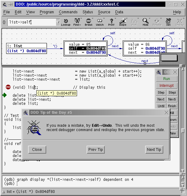
- DDD : Data Display Debugger
Although dated, its great strenght is the ability to plot data with the command
grap plot dataarrayname, and check its evilution as the you debug. - Others
Codeblocks, geany, clion, etc all them have interfaces for gdb.
- Online gdb
7.3.7. Another exercise
Please try to help the poor code called please_fixme.cpp. Share your
experiences. How many bugs did you find?
#Poor man’s profiler#
- Get the process id:
$ top
or
$ ps aux
- Attach the process to gdb (
PIDis the process id):
$ gdb -p PID
Now the program is paused.
- check the stack:
(gdb) thread apply all bt
Check what appears first.
- Continue the execution:
(gdb) continue
- Repeat previous two steps as many times as you want and make a histogram of the most executed functions.
7.3.8. Debugging within emacs
Please check emacs gdb mode
- Open your source code with emacs.
- Compile with
M-x compile.Mis the meta function. By default it uses make, but you can modify the compile command. - Activate de debugging:
M-x gdb - Debug. To move from one frame to another you can use either the mouse
or the shortcut
ctrl-x o. To close a pane, usectrl-x 0when inside that pane.
7.3.9. Modern tools
- Python
Gdb version >= 7.x supports python. You can use to explore more info about your program, pretty print data, and even plot (although blocking).
To load a c++ var into a python do, inside gdb,
    py my_array = gdb.parse_and_eval("my_array")
    py print my_array.type
Even more, to plot some data structure with matplotlib, you can as follows (Based on https://blog.semicolonsoftware.de/debugging-numerical-c-c-fortran-code-with-gdb-and-numpy/)
 1:   int main(int argc, char **argv) {
 2:     const int nrow = 4;
 3:     const int ncol = 3;
 4:     double x[nrow * ncol];
 5:     for(int i = 0; i < nrow; i++) {
 6:       for(int j = 0; j < ncol; j++) {
 7:     x[i * ncol + j]  = i * j;
 8:       }
 9:     }
10:     // BREAK here
11:   }
Follow the previous url to install gdbnumpy.py.
Compile as
gcc ex-01.c -g -ggdb
and now, run
gdband put the following commandsbr 10 # sets a breakpoint run # to load the program symbols py import gdb_numpy py x = gdb_numpy.to_array("(double *)x", shape=(4 * 3,)).reshape(4, 3) py print x py import matplotlib.pyplot as plt py plt.imshow(x) py plt.show()
Use gdb to execute, step by step, the following code
#include <iostream>
#include <cstdlib>

int main(int argc, char **argv)
{
    int a;
    a = 0;
    std::cout << a << std::endl;
    a = 5;

    return EXIT_SUCCESS;
}
7.3.10. Examples to debug
Example 1
#include <iostream>

int main(void)
{
  //double x[10], y[5]; // imprime raro
  double y[5], x[10]; // imprime 1

  for(int ii = 0; ii < 5; ++ii) {
    y[ii] = ii +1;
  }
  for(int ii = 0; ii < 10; ++ii) {
    x[ii] = -(ii +1);
  }

  double z = x[10];
  std::cout << z << std::endl;

  return 0;
}
7.4. DDD : Data Display Debugger
The Data Display Debugger - ddd is a graphical frontend for command line debuggers like gdb, dbx, jdb, bashdb, etc, and some modified python debugger. It easies the debug processing by adding some capabilities, like visual monitoring of data and data plotting (killer feature).
NOTE: DDD is hard to configure, it is so rebel. If after configuring some options you are having issues, like dd hanging with a message “Waiting for gdb to start”, or the plotting window is always waiting, then close ddd, delete the config file with
rm -rf ~/.ddd, and start over by configuring ONLY one option at a time (configure one option, then close it, then open, then configure other option, then close, etc).
7.4.1. Exercise
Repeat the previous debugging exercises by using ddd. In particular, use
the display and watch. Do you find them convenient? and what about
graph display data?
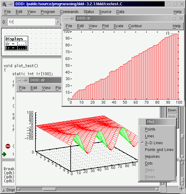
7.4.2. DDD data plotting with gnuplot
One of the killer features of ddd is its capability to actually plot the data with gnuplot. Let’s do an example:
- Compile (with debugging activated, of course) the code
array.cpp. - Now open the executable with ddd.
- Establish a break point at main.
- Run the executable under ddd.
- Now write
graph plot data, or equivalently, you can selectdatawith the mouse and then click to plot on the menu bar. NOTE : If you are having issues please try to configure gnuplot helper to be on an external window, then close, then re-open, and try again. Check also Notes above. - Now proceed by steps. You will be able to see a plot of the array
dataas it changes its values. Awesome, isn’t it? - Do the same for the 2d array. What will you expect now to be plotted? a line or a surface?
7.5. TODO Examples to solve
Let’s use ddd to explore some other exercises.
- ICTP examples
Browse to ICTP-examples, then go to debugging, then ICTP-gdbexamples , and download each file, or just download all files compressed at example files
- Other
These are more examples: original link
7.6. Valgrind

Figure 1: Valgrind Logo
From Web Page: > Valgrind is an instrumentation framework for building dynamic analysis tools. There are Valgrind tools that can automatically detect many memory management and threading bugs, and profile your programs in detail. You can also use Valgrind to build new tools.
The Valgrind distribution currently includes six production-quality tools: a memory error detector, two thread error detectors, a cache and branch-prediction profiler, a call-graph generating cache and branch-prediction profiler, and a heap profiler. It also includes three experimental tools: a heap/stack/global array overrun detector, a second heap profiler that examines how heap blocks are used, and a SimPoint basic block vector generator. It runs on the following platforms: X86/Linux, AMD64/Linux, ARM/Linux, PPC32/Linux, PPC64/Linux, S390X/Linux, MIPS/Linux, ARM/Android (2.3.x and later), X86/Android (4.0 and later), X86/Darwin and AMD64/Darwin (Mac OS X 10.6 and 10.7, with limited support for 10.8).
7.6.1. Graphical Interfaces
7.6.2. As memory checker
In this section we will focus on valgrind as memory checker tool (debugging part). Therefore, we will invoke valgrind with that option:
$ valgrind --tool=memcheck --leak-check=yes myprog arg1 arg2
where myprog is your executable’s name, and arg1 etc are the
arguments.
We will use the files inside valgrind/Valgrind-QuickStart
Please compile the file a.c (which is also on the compressed file -
check wiki main page) and run valgrind on it. What do you obtain? Do you
have memory leaks? Please fix it until you have no memory errors.
Do the same for b.c .
- Example : Memory leak
#include <iostream>
#include <cstdlib>

void getmem(double *ptr, int n);

int main(int argc, char **argv)
{
  // declare variables
  const int N = 10000;
  double * array;
  for (int ii = 0 ; ii < 20; ++ii) {
    getmem(array, N);
  }
  // free memory
  // delete [] array;

  return EXIT_SUCCESS;
}

void getmem(double *ptr, int n)
{
  ptr = new double [n];
  data[0] = data[1]*2;
}
- More examples : ICTP
https://github.com/thehackerwithin/PyTrieste/tree/master/valgrind
Please enter the
SoftwareCarpentry-ICTPvalgrind subfolder and locate the source files. CompilesimpleTest.ccas$ g++ -g simpleTest.cc -o simpleTest
Now run valgrind on it
$ valgrind --track-origins=yes --leak-check=full ./simpleTest 300 300
Check how the memory leaks depend on the parameters. Fix the code.
7.7. TODO Homework
Modularize one of the previous codes into a header a implementation file and a main file. This will help when writing tests.
8. Unit Testing : Ensuring fix and correct behavior last
Unity testing allows to ensure that a given software behaves in the correct way, at least for the cases one is testing. Once a function is written (or even before in TTD) or a bug is fixed, it is necessary to write a test that ensures the function to work properly in limit cases or the bug to not reappear in the future. There are several levels associated with unit testing .
In this unit we will learn the general philosophy behind it and a couple of tools to implement very basic tests, althoguh the list of testing frameworks is very large. Furthermore, modularization will be very important, so you must have a clear understanding on how to split some given code into headers, source files, and how to compile objects and then link them using the linker, hopefully through a Makefile.
8.1. Catch2
Our goal here is to learn to use catch2 to test a very simple function extracted
from their tutorial. Later we will modularize the code to practice that and
write a useful Makefile.
8.1.1. Install catch2
We will install catch2 using spack:
spack install catch2
8.1.2. Tutorial example
This is the file example extracted from catch2 tutorial.
#define CATCH_CONFIG_MAIN  // This tells Catch to provide a main() - only do this in one cpp file
#include "catch2/catch.hpp"
//#include "catch.hpp"

unsigned int Factorial( unsigned int number ) {
  return number <= 1 ? number : Factorial(number-1)*number;
}

TEST_CASE( "Factorials are computed", "[factorial]" ) {
  REQUIRE( Factorial(1) == 1 );
  REQUIRE( Factorial(2) == 2 );
  REQUIRE( Factorial(3) == 6 );
  REQUIRE( Factorial(10) == 3628800 );
}
Catch is header only. Compile this as
g++ example_test.cpp
then run the executable and the tests info will be presented on the screen.
Can you see if there is a bug in the factorial code? fix it and add
a test REQUIRE in the same file.
8.1.3. Code modularization
Modularization allows us to split the implementation, the interface, and the test.
To modularize the code we need to take the only function here, factorial, and
split it into a header and source file:
header file:
#pragma once
int factorial(int n);
Implementation file:
#include "factorial.h"

int factorial(int number)
{
return number <= 1 ? number : factorial(number-1)*number;
}
Clearly this factorial.cpp file cannot be compiled into and
executable since it does no contain a main function. But it can be
used to construct and object file (flag -c on the compiler) to
later link with other object files.
Now we create a main file that will call the factorial function:
#include <iostream>
#include "factorial.h"

int main(void)
{
  std::cout << factorial(4) << std::endl;
  return 0;
}
And then compile it as
g++ -c factorial.cpp # creates factorial.o that can be used for the testing
g++ -c factorial_main.cpp # creates main_factorial.o
g++ factorial.o factorial_main.o -o main_factorial.x # links and creates executable
./main_factorial.x
8.1.4. Writing the test
Let’s first write the test
#define CATCH_CONFIG_MAIN  // This tells Catch to provide a main() - only do this in one cpp file
#include "catch2/catch.hpp"

#include "factorial.h"

TEST_CASE( "Factorials are computed", "[factorial]" ) {
    //REQUIRE( factorial(0) == 1 );
    REQUIRE( factorial(1) == 1 );
    REQUIRE( factorial(2) == 2 );
    REQUIRE( factorial(3) == 6 );
    REQUIRE( factorial(10) == 3628800 );
}
Now let’s run the test using the modularized code. First, let’s load catch
spack load catch2
Compile and execute as
g++ -c factorial.cpp
g++ -c factorial_test.cpp
g++ factorial.o factorial_test.o -o factorial_test.x
./factorial_test.x
Now you can test or run-with-not-tests independently.
8.1.5. Makefile
To compile this and future tests, is useful to implement all in a Makefile
SHELL:=/bin/bash

all: factorial_main.x

test: factorial_test.x
    ./$<

%.x: %.o factorial.o
    source $$HOME/repos/spack/share/spack/setup-env.sh; \
    spack load catch2; \
    g++ $$(pkg-config --cflags catch2) $^ -o $@

%.o: %.cpp
    source $$HOME/repos/spack/share/spack/setup-env.sh; \
    spack load catch2; \
    g++ $$(pkg-config --cflags catch2) -c $<

clean:
    rm -f *.o *.x
8.2. google test
Google test is a famous and advance unit framework that goes well beyond of what is shown here. You are invited to follow the docs to learn more.
8.2.1. Installation
Again, we will use spack
spack install googletest
mkdir googletest
8.2.2. Example
This is an example, already modularized.
- Factorial and isprime header:
#ifndef GTEST_SAMPLES_SAMPLE1_H_
#define GTEST_SAMPLES_SAMPLE1_H_

// Returns n! (the factorial of n).  For negative n, n! is defined to be 1.
int Factorial(int n);

//// Returns true if and only if n is a prime number.
bool IsPrime(int n);

#endif  // GTEST_SAMPLES_SAMPLE1_H_
- Source file
#include "factorial.h"

// Returns n! (the factorial of n).  For negative n, n! is defined to be 1.
    int Factorial(int n) {
    int result = 1;
    for (int i = 1; i <= n; i++) {
        result *= i;
    }

    return result;
  }

// Returns true if and only if n is a prime number.
bool IsPrime(int n) {
    // Trivial case 1: small numbers
    if (n <= 1) return false;

    // Trivial case 2: even numbers
    if (n % 2 == 0) return n == 2;

    // Now, we have that n is odd and n >= 3.

    // Try to divide n by every odd number i, starting from 3
    for (int i = 3; ; i += 2) {
        // We only have to try i up to the square root of n
        if (i > n/i) break;

        // Now, we have i <= n/i < n.
        // If n is divisible by i, n is not prime.
        if (n % i == 0) return false;
    }

    // n has no integer factor in the range (1, n), and thus is prime.
    return true;
}
- Test source file (to be compiled as an object)
#include <limits.h>
#include "factorial.h"
#include "gtest/gtest.h"
namespace {
    // Tests factorial of negative numbers.
    TEST(FactorialTest, Negative) {
        // This test is named "Negative", and belongs to the "FactorialTest"
        // test case.
        EXPECT_EQ(1, Factorial(-5));
        EXPECT_EQ(1, Factorial(-1));
        EXPECT_GT(Factorial(-10), 0);
    }
    // Tests factorial of 0.
    TEST(FactorialTest, Zero) {
        EXPECT_EQ(1, Factorial(0));
    }

// Tests factorial of positive numbers.
    TEST(FactorialTest, Positive) {
        EXPECT_EQ(1, Factorial(1));
        EXPECT_EQ(2, Factorial(2));
        EXPECT_EQ(6, Factorial(3));
        EXPECT_EQ(40320, Factorial(8));
    }

    // Tests negative input.
    TEST(IsPrimeTest, Negative) {
        // This test belongs to the IsPrimeTest test case.

        EXPECT_FALSE(IsPrime(-1));
        EXPECT_FALSE(IsPrime(-2));
        EXPECT_FALSE(IsPrime(INT_MIN));
    }

// Tests some trivial cases.
    TEST(IsPrimeTest, Trivial) {
        EXPECT_FALSE(IsPrime(0));
        EXPECT_FALSE(IsPrime(1));
        EXPECT_TRUE(IsPrime(2));
        EXPECT_TRUE(IsPrime(3));
    }

// Tests positive input.
    TEST(IsPrimeTest, Positive) {
        EXPECT_FALSE(IsPrime(4));
        EXPECT_TRUE(IsPrime(5));
        EXPECT_FALSE(IsPrime(6));
        EXPECT_TRUE(IsPrime(23));
    }
}
- Main google test file
#include <cstdio>
#include "gtest/gtest.h"

GTEST_API_ int main(int argc, char **argv) {
    printf("Running main() from %s\n", __FILE__);
    testing::InitGoogleTest(&argc, argv);
    return RUN_ALL_TESTS();
}
9. Profiling
After debugging your code and writing several tests to avoid repeating the same bug, you want to start optimizing it to make it fast (but keeping it correct). To do this, you need to measure. You need to detect functions which take most of the time. Optimizing a function that takes only 5% of the time will give you only marginal benefits. Finding the functions that take most of the time is called profiling , and there are several tools ready to help you. In the following we ill learn to use these tools to detect the hotspots/bottlenecks in our codes.
9.1. Why profile?
Profiling allows you to learn how the computation time was spent and how the data flows in your program. This can be achieved by just printing the time spent on each section using some internal timers, or, better, by using a tool called “profiler” that shows you how time was spent in your program and which functions called which other functions.
Using a profiler is something that comes very handy when you want to verify that your program does what you want it to do, especially when it is not easy to analyze (it may contain many functions or many calls to different functions and so on).
Remember, WE ARE SCIENTISTS, so we want to profile code to optimize the computation time taken by our program. The key idea then becomes finding where (which function/subroutine) is the computation time spent and attack it using optimization techniques (studied in a previous session of this course, check this).
9.2. Measuring elapsed time
The first approach is to just add timers to your code. This is a good practice and it is useful for a code to report the time spent on different parts. The following example is extracted from here and modified to make it a bit simpler:
#include <cstdio>
#include <cstdlib>

/*
  Tests cache misses.
*/

int main(int argc, char **argv)
{
  if (argc < 3){
    printf("Usage: cacheTest sizeI sizeJ\nIn first input.\n");
    return 1;
  }
  long sI = atoi(argv[1]);
  long sJ = atoi(argv[2]);

  printf("Operating on matrix of size %ld by %ld\n", sI, sJ);

  long *arr = new long[sI*sJ]; // double array.

  // option 1
  for (long i=0; i < sI; ++i)
    for (long j=0; j < sJ; ++j)
      arr[(i * (sJ)) + j ] = i;

  // option 2
  for (long i=0; i < sI; ++i)
    for (long j=0; j < sJ; ++j)
      arr[(j * (sI)) + i ] = i;

  // option 3
  for (int i=0; i < sI*sJ; ++i) arr[i] = i;

  printf("%ld\n", arr[0]);

  return 0;
}
Now let’s add some timers using the chrono c++11 library (you can see more
eamples here and here .
#include <cstdio>
#include <cstdlib>
#include <chrono>
#include <iostream>

/*
   Tests cache misses.
*/

template <typename T>
void print_elapsed(T start, T end );

int main(int argc, char **argv)
{
  if (argc < 3){
    printf("Usage: cacheTest sizeI sizeJ\nIn first input.\n");
    return 1;
  }
  long sI = atoi(argv[1]);
  long sJ = atoi(argv[2]);

  printf("Operating on matrix of size %ld by %ld\n", sI, sJ);

  auto start = std::chrono::steady_clock::now();
  long *arr = new long[sI*sJ]; // double array.
  auto end = std::chrono::steady_clock::now();
  print_elapsed(start, end);

  // option 1
  start = std::chrono::steady_clock::now();
  for (long i=0; i < sI; ++i)
    for (long j=0; j < sJ; ++j)
      arr[(i * (sJ)) + j ] = i;
  end = std::chrono::steady_clock::now();
  print_elapsed(start, end);

  // option 2
  start = std::chrono::steady_clock::now();
  for (long i=0; i < sI; ++i)
      for (long j=0; j < sJ; ++j)
         arr[(j * (sI)) + i ] = i;
  end = std::chrono::steady_clock::now();
  print_elapsed(start, end);

  // option 3
  start = std::chrono::steady_clock::now();
  for (int i=0; i < sI*sJ; ++i) arr[i] = i;
  end = std::chrono::steady_clock::now();
  print_elapsed(start, end);

  printf("%ld\n", arr[0]);

  return 0;
}

template <typename T>
void print_elapsed(T start, T end )
{
  std::cout << "Elapsed time in ms: "
        << std::chrono::duration_cast<std::chrono::milliseconds>(end-start).count()
        << "\n";
}
Analyze the results.
9.3. Profilers
There are many types of profilers from many different sources, commonly, a profiler is associated to a compiler, so that for example, GNU (the community around gcc compiler) has the profiler ’gprof’, intel (corporation behind icc) has iprof, PGI has pgprof, etc. Valgrind is also a useful profiler through the cachegrind tool, which has been shown at the debugging section.
This crash course (more like mini tutorial) will focus on using gprof. Note that gprof supports (to some extend) compiled code by other compilers such as icc and pgcc. At the end we will briefly review perf, and the google performance tools.
FACT 1: According to Thiel, “gprof … revolutionized the performance analysis field and quickly became the tool of choice for developers around the world …, the tool is still actively maintained and remains relevant in the modern world.” (from Wikipedia).
FACT 2: Top 50 most influential papers on PLDI (from Wikipedia).
9.4. gprof
Inthe following we will use the following code as example:
Example 1: Basic gprof (compile with gcc)
//test_gprof.c
#include<stdio.h>

void new_func1(void);
void func1(void);
static void func2(void);
void new_func1(void);

int main(void)
{
  printf("\n Inside main()\n");
  int i = 0;

  for(;i<0xffffff;i++);
  func1();
  func2();

  return 0;
}
void new_func1(void);

void func1(void)
{
  printf("\n Inside func1 \n");
  int i = 0;

  for(;i<0xffffffff;i++);
  new_func1();

  return;
}

static void func2(void)
{
  printf("\n Inside func2 \n");
  int i = 0;

  for(;i<0xffffffaa;i++);
  return;
}

void new_func1(void)
{
  printf("\n Inside new_func1()\n");
  int i = 0;

  for(;i<0xffffffee;i++);

  return;
}
Para usar gprof:
Compilar con
-pggcc -Wall -pg -g test_gprof.c -o test_gprof
Ejecutar normalmente. Esto crea o sobreescribe un archivo
gmon.out./test_gprof
Abrir el reporte usando
gprof test_gprof gmon.out > analysis.txt
This produces a file called ’analysis.txt’ which contains the profiling information in a human-readable form. The output of this file should be something like the following:
  Flat profile:

  Each sample counts as 0.01 seconds.
    %   cumulative   self              self     total
   time   seconds   seconds    calls   s/call   s/call  name
   39.64      9.43     9.43        1     9.43    16.79  func1
   30.89     16.79     7.35        1     7.35     7.35  new_func1
   30.46     24.04     7.25        1     7.25     7.25  func2
    0.13     24.07     0.03                             main

   %         the percentage of the total running time of the
  time       program used by this function.

  cumulative a running sum of the number of seconds accounted
   seconds   for by this function and those listed above it.

   self      the number of seconds accounted for by this
  seconds    function alone.  This is the major sort for this
             listing.

  calls      the number of times this function was invoked, if
             this function is profiled, else blank.

   self      the average number of milliseconds spent in this
  ms/call    function per call, if this function is profiled,
         else blank.

   total     the average number of milliseconds spent in this
  ms/call    function and its descendents per call, if this
         function is profiled, else blank.

  name       the name of the function.  This is the minor sort
             for this listing. The index shows the location of
         the function in the gprof listing. If the index is
         in parenthesis it shows where it would appear in
         the gprof listing if it were to be printed.

               Call graph (explanation follows)


  granularity: each sample hit covers 2 byte(s) for 0.04% of 24.07 seconds

  index % time    self  children    called     name
                                                   <spontaneous>
  [1]    100.0    0.03   24.04                 main [1]
                  9.43    7.35       1/1           func1 [2]
                  7.25    0.00       1/1           func2 [4]
  -----------------------------------------------
                  9.43    7.35       1/1           main [1]
  [2]     69.7    9.43    7.35       1         func1 [2]
                  7.35    0.00       1/1           new_func1 [3]
  -----------------------------------------------
                  7.35    0.00       1/1           func1 [2]
  [3]     30.5    7.35    0.00       1         new_func1 [3]
  -----------------------------------------------
                  7.25    0.00       1/1           main [1]
  [4]     30.1    7.25    0.00       1         func2 [4]
  -----------------------------------------------

   This table describes the call tree of the program, and was sorted by
   the total amount of time spent in each function and its children.

   Each entry in this table consists of several lines.  The line with the
   index number at the left hand margin lists the current function.
   The lines above it list the functions that called this function,
   and the lines below it list the functions this one called.
   This line lists:
       index  A unique number given to each element of the table.
          Index numbers are sorted numerically.
          The index number is printed next to every function name so
          it is easier to look up where the function is in the table.

       % time This is the percentage of the `total' time that was spent
          in this function and its children.  Note that due to
          different viewpoints, functions excluded by options, etc,
          these numbers will NOT add up to 100%.

       self   This is the total amount of time spent in this function.

       children   This is the total amount of time propagated into this
          function by its children.

       called This is the number of times the function was called.
          If the function called itself recursively, the number
          only includes non-recursive calls, and is followed by
          a `+' and the number of recursive calls.

       name   The name of the current function.  The index number is
          printed after it.  If the function is a member of a
          cycle, the cycle number is printed between the
          function's name and the index number.


   For the function's parents, the fields have the following meanings:

       self   This is the amount of time that was propagated directly
          from the function into this parent.

       children   This is the amount of time that was propagated from
          the function's children into this parent.

       called This is the number of times this parent called the
          function `/' the total number of times the function
          was called.  Recursive calls to the function are not
          included in the number after the `/'.

       name   This is the name of the parent.  The parent's index
          number is printed after it.  If the parent is a
          member of a cycle, the cycle number is printed between
          the name and the index number.

   If the parents of the function cannot be determined, the word
   `<spontaneous>' is printed in the `name' field, and all the other
   fields are blank.

   For the function's children, the fields have the following meanings:

       self   This is the amount of time that was propagated directly
          from the child into the function.

       children   This is the amount of time that was propagated from the
          child's children to the function.

       called This is the number of times the function called
          this child `/' the total number of times the child
          was called.  Recursive calls by the child are not
          listed in the number after the `/'.

       name   This is the name of the child.  The child's index
          number is printed after it.  If the child is a
          member of a cycle, the cycle number is printed
          between the name and the index number.

   If there are any cycles (circles) in the call graph, there is an
   entry for the cycle-as-a-whole.  This entry shows who called the
   cycle (as parents) and the members of the cycle (as children.)
   The `+' recursive calls entry shows the number of function calls that
   were internal to the cycle, and the calls entry for each member shows,
   for that member, how many times it was called from other members of
   the cycle.


  Index by function name

     [2] func1                   [1] main
     [4] func2                   [3] new_func1
The output has two sections: >*Flat profile:* The flat profile shows the total amount of time your program spent executing each function.
Call graph: The call graph shows how much time was spent in each function and its children.
9.5. perf
9.5.1. Installing perf
Perf is a kernel module, so you will need to install it from the kernel source. As root, the command used to install perl in the computer room was
cd /usr/src/linux/tools/perf/; make -j $(nproc); cp perf /usr/local/bin
This will copy the perf executable into the path.
9.5.2. Using perf
Perf is a hardware counter available on linux platforms.
Its use is very simple: Just run, For a profile summary,
perf stat ./a.out > profile_summary
For gprof-like info, use
perf record ./a.out
perf report
9.5.3. Hotstop: Gui for perf
https://github.com/KDAB/hotspot Install with the appimage: Download it, make it executable, run.
In the computer room you can also use spack:
spack load hotspot-perf
And then just use the command hotspot .
9.6. Profiling with valgrind: cachegrind and callgrind
Valgrind allows not only to debug a code but also to profile it. Here we will see how to use cachegrind, to check for cache misses, and callgrind, for a calling graph much like tools like perf and gprof.
9.6.1. Cache checker : cachegrind
From cachegrind
Cachegrind simulates how your program interacts with a machine'scache hierarchy and (optionally) branch predictor. It simulates a machine with independent first-level instruction and data caches (I1 and D1), backed by a unified second-level cache (L2). This exactly matches the configuration of many modern machines.
However, some modern machines have three levels of cache. For these machines (in the cases where Cachegrind can auto-detect the cache configuration) Cachegrind simulates the first-level and third-level caches. The reason for this choice is that the L3 cache has the most influence on runtime, as it masks accesses to main memory. Furthermore, the L1 caches often have low associativity, so simulating them can detect cases where the code interacts badly with this cache (eg. traversing a matrix column-wise with the row length being a power of 2).
Therefore, Cachegrind always refers to the I1, D1 and LL (last-level) caches.
To use cachegrind, you will need to invoke valgrind as
valgrind --tool=cachegrind prog
Take into account that execution will be (possibly very) slow.
Typical output:
  ==31751== I   refs:      27,742,716
  ==31751== I1  misses:           276
  ==31751== LLi misses:           275
  ==31751== I1  miss rate:        0.0%
  ==31751== LLi miss rate:        0.0%
  ==31751==
  ==31751== D   refs:      15,430,290  (10,955,517 rd + 4,474,773 wr)
  ==31751== D1  misses:        41,185  (    21,905 rd +    19,280 wr)
  ==31751== LLd misses:        23,085  (     3,987 rd +    19,098 wr)
  ==31751== D1  miss rate:        0.2% (       0.1%   +       0.4%)
  ==31751== LLd miss rate:        0.1% (       0.0%   +       0.4%)
  ==31751==
  ==31751== LL misses:         23,360  (     4,262 rd +    19,098 wr)
  ==31751== LL miss rate:         0.0% (       0.0%   +       0.4%)
The output and more info will be written to cachegrind.out.<pid>,
where pid is the PID of the process. You can open that file with
valkyrie for better analysis.
The tool cg_annonate allows you postprocess better the file
cachegrind.out.<pid>.
Compile the file cacheTest.cc,
$ g++ -g cacheTest.cc -o cacheTest
Now run valgrind on it, with cache checker
$ valgrind --tool=cachegrind ./cacheTest 0 1000 100000
Now let’s check the cache-misses per line of source code:
cg_annotate --auto=yes cachegrind.out.PID
where you have to change PID by the actual PID in your results.
Fix the code.
- More cache examples
Please open the file
cache.cppwhich is inside the directory valgrind. Read it. Comment the linestd::sort(data, data + arraySize);
Compile the program and run it, measuring the execution time (if you wish, you can use optimization):
  $ g++ -g cache.cpp -o cache.x
  $ time ./cache.x
The output will be something like
  26.6758
  sum = 312426300000

  real    0m32.272s
  user    0m26.560s
  sys 0m0.122s
Now uncomment the same line, re-compile and re-run. You will get something like
  5.37881
  sum = 312426300000

  real    0m6.180s
  user    0m5.360s
  sys 0m0.026s
The difference is big. You can verify that this happens even with compiler optimisations enabled. What it is going on here?
Try to figure out an explanation before continuing.
Now let’s use valgrind to track the problem. Run the code (with the sort line commented) with cachegrind:
$ valgrind --tool=cachegrind ./a.out
And now let’s annotate the code (remember to change PID for your actual number):
cg_annonate --auto=yes cachegrind.out.PID
We can see that we have something similar to stackoverflow analysis
Understand why.
9.6.2. Callgrind
Now, we are using valgrind to get a calling
profile by using the tool callgrind. It is done as follows: Use
the same programa as in other modules. First, compile with debugging
enabled, something like
gcc -g -ggdb name.c -o name.x
and now execute with valgrind as
valgrind --tool=callgrind name.x [possible options]
Results will be stored on the files callgrind.out.PID, where PID
is the process identifier.
You can read the previous file with a text editor, by using the instructions
callgrind_annotate --auto=yes callgrind.out.PID
and you can also use the tool KCachegrind,
kcachegrind callgrind.out.PID
(do not forget to replace PID by the actual number). The first view presents the list of the profiled functions. If you click on a function, other views appear with more info, as callers, calling map, source code, etc.
NOTE: If you want to see correct function names, you can use the command
valgrind --tool=callgrind --dump-instr=yes --collect-jumps=yes ./program program_parameters
Please run and use callgrind to study the previous programs and also a program using eigen library. In the later, it is easy to profile?
9.7. Google Performance Tools
See https://github.com/gperftools/gperftools
From Google performance tools : These tools are for use by developers so that they can create more robust applications. Especially of use to those developing multi-threaded applications in C++ with templates. Includes TCMalloc, heap-checker, heap-profiler and cpu-profiler.
In brief:
  TC Malloc:

  gcc [...] -ltcmalloc
  Heap Checker:

  gcc [...] -o myprogram -ltcmalloc
  HEAPCHECK=normal ./myprogram
  Heap Profiler:

  gcc [...] -o myprogram -ltcmalloc
  HEAPPROFILE=/tmp/netheap ./myprogram
  Cpu Profiler:

  gcc [...] -o myprogram -lprofiler
  CPUPROFILE=/tmp/profile ./myprogram
Basically, when ypu compile, you link with the required library. Then, you can generate a callgraph with profiler info. Try to install the google performance tool on your home and test them with the previous codes. Please review the detailed info for each tool: for example, for the cpu profiler, check Cpu profiler info
9.8. Exercises
- Take this code and modify it (separate its behaviour into functions) to be able to profile it.
- Download https://bitbucket.org/iluvatar/scientific-computing-part-01/downloads/CodigosIvan.zip, run , and optimize them.
- Experiment: Take this code, profile it and try to optimize it in any way.
10. Optimization
First of all :
Programmers waste enormous amounts of time thinking about, or worrying about,the speed of noncritical parts of their programs, and these attempts at efficiency actually have a strong negative impact when debugging and maintenance are considered. We should forget about small efficiencies, say about 97% of the time: premature optimization is the root of all evil. Yet we should not pass up our opportunities in that critical 3%. Donald Knuth
First, make your program correct, then measure, then optimize. Optimization can be achieved by just using compiler flags, by using already optimized libraries, and sometimes by being careful with our memory usage. Some low level techniques are better left to the compiler.
10.1. Compiler flags
See : https://gcc.gnu.org/onlinedocs/gcc/Optimize-Options.html
Sometimes just using compiler optimization flags with can improve dramatically our code performance. Normally, you want to run your code through several compiler flags to check for speed ups but also for possible uncovered bugs.
Compile without (-O0) and with optimization (-O3) the following code and
compare their runtime:
// Credits : Ivan Pulido
/* Shows a way to do operations that require a specific order (e.g.,
 * transpositions) while avoiding cache misses. */

#include <stdio.h>
#include <time.h>
#include <stdlib.h>

#define min( a, b ) ( ((a) < (b)) ? (a) : (b) )

int main(){
    const int n = 512;
    const int csize = 32;
    float ***a, ***b;
    clock_t cputime1, cputime2;
    int i,j,k,ii,jj,kk;

    // Allocating memory for array/matrix
    a = malloc(n*sizeof(float **));
    for (i=0; i<n; i++){
        a[i] = malloc(n*sizeof(float*));
        for (j=0; j<n; j++)
            a[i][j] = malloc(n*sizeof(float));
    }
    b = malloc(n*sizeof(float **));
    for (i=0; i<n; i++){
        b[i] = malloc(n*sizeof(float*));
        for (j=0; j<n; j++)
            b[i][j] = malloc(n*sizeof(float));
    }

    // Filling matrices with zeros
    for(i=0; i<n; ++i)
        for (j=0; j<n; ++j)
            for (k=0; k<n; ++k)
                a[i][j][k] = 0;
    for(i=0; i<n; ++i)
        for (j=0; j<n; ++j)
            for (k=0; k<n; ++k)
                b[i][j][k] = 0;

    // Direct (inefficient) transposition
    cputime1 = clock();
    for (i=0; i<n; ++i)
        for (j=0; j<n; ++j)
            for (k=0; k<n; ++k)
                a[i][j][k] = b[k][j][i];
    cputime2 = clock() - cputime1;
    printf("Time for transposition: %f\n", ((double)cputime2)/CLOCKS_PER_SEC);

    // Transposition using cache-blocking
    cputime1 = clock();
    for (ii=0; ii<n; ii+=csize)
        for (jj=0; jj<n; jj+=csize)
            for (kk=0; kk<n; kk+=csize)
                for (i=ii; i<min(n,ii+csize-1); ++i)
                    for (j=jj; j<min(n,jj+csize-1); ++j)
                        for (k=kk; k<min(n,kk+csize-1); ++k)
                            a[i][j][k] = b[k][j][i];
    cputime2 = clock() - cputime1;
    printf("Time for transposition: %f\n", ((double)cputime2)/CLOCKS_PER_SEC);

    return 0;
}
When you compile without optimization and execute, you will get something like
gcc -O0 cache_blocking.c
./a.out
| Time | for | transposition: | 0.149666 |
| Time | for | transposition: | 0.079659 |
But, if you use optimization, you can get an important improvement
gcc -O2 cache_blocking.c
./a.out
| Time | for | transposition: | 0.249758 |
| Time | for | transposition: | 0.063044 |
Actually we can compare all optimization levels to check their impact:
for level in 0 1 2 3; do echo "level: $level"; gcc -O$level cache_blocking.c; ./a.out; done
| level: | 0 | ||
| Time | for | transposition: | 0.458889 |
| Time | for | transposition: | 0.165291 |
| level: | 1 | ||
| Time | for | transposition: | 0.227113 |
| Time | for | transposition: | 0.066454 |
| level: | 2 | ||
| Time | for | transposition: | 0.256035 |
| Time | for | transposition: | 0.062626 |
| level: | 3 | ||
| Time | for | transposition: | 0.217729 |
| Time | for | transposition: | 0.055846 |
Be careful when using -O3: it activates some unsafe math optimizations that will
not respect IEEE754.
10.2. Memory layout
The memory layout should always be taken into account since cache misses will greatly affect a program performance. Always measure with a profiler and if possible with cachegrind in order to detect possible excessive cache misses.
The following code shows how a simple index change in a matrix operation could have a huge impact on the app performance:
// Credit Ivan Pulido
#include <stdio.h>
#include <stdlib.h>
#include <time.h>

int main(){
    const int n = 256;
    clock_t cputime1, cputime2;
    float ***a;
    int i,j,k;

    // Allocating memory for array/matrix
    a = malloc(n*sizeof(float **));
    for (i=0; i<n; i++){
        a[i] = malloc(n*sizeof(float*));
        for (j=0; j<n; j++)
            a[i][j] = malloc(n*sizeof(float));
    }
    cputime1 = clock();
    for (k=0; k<n; ++k)
        for (j=0; j<n; ++j)
            for (i=0; i<n; ++i)
                a[i][j][k] = 1.0;
    cputime2=clock() - cputime1;
    printf("Time with fast index inside: %lf\n", ((double)cputime2)/CLOCKS_PER_SEC);

    cputime1 = clock();
    for(i=0; i<n; ++i)
        for (j=0; j<n; ++j)
            for (k=0; k<n; ++k)
                a[i][j][k] = 2.3;
    cputime2=clock() - cputime1;
    printf("Time with fast index outside: %lf\n", ((double)cputime2)/CLOCKS_PER_SEC);

    // Clearing memory
    for (i=0; i<n; i++){
        for (j=0; j<n; j++)
            free(a[i][j]);
        free(a[i]);
    }
    free(a);

    return 0;
}
gcc codes/cache_lines.c
./a.out
| Time | with | fast | index | inside: | 0.139432 |
| Time | with | fast | index | outside: | 0.027866 |
Being nice to the cache comes from the modern cpu architecture, as shown in the next figure

Figure 2: L1, L2 and L3 caches. Source https://medium.com/software-design/why-software-developers-should-care-about-cpu-caches-8da04355bb8a
The relative bandwidth across the different cpu and momory controllers explain why it is important to have the processed data as much time as possible in the cache

Figure 3: Relative bandwidth across different cpu and computer parts. Credit: https://cs.brown.edu/courses/csci1310/2020/assign/labs/lab4.html
Since c/c++ store matrices in row major order, then accesing the memory in the same way will benefit the cache and therefore increases our program performance.
10.2.1. What data structures to use?
It depends greatly from the problem. But for the typical applications of vector
and matrix computations, we can expect that homogeneous and contiguous arrays
are the data structures to go. In that case, it is advisable to use
std::vector as the go to data struct since it is as efficient as an primitive
arra, handles automatically the dynamic memory in the heap, and plays nice with
the C++ STL.
A primitive static array is limited by the stack. Play with the values of M and N in the following code until you get a seg fault just by running the code.
#include <iostream>

int main(void)
{
    const int M = 7000;
    const int N = 500;
    double data[M][N] = {{0.0}};

    std::cout << data[M/2][N/2] << std::endl;

    return 0;
}
Is the maximum size related somehow with the output of the command ulimit -s ?
To be able to use more memory, you could better use dynamic memory with
primitive arrays, but you will have to manage the new/delete parts in your
code. Check that foloowing code does not die on the same sizes as the previous
one
#include <iostream>

int main(void)
{
    const int M = 7000;
    const int N = 500;

    double **data = nullptr;
    data = new double *[M];
    for (int ii = 0; ii < M; ++ii){
        data[ii] = new double [N];
    }

    std::cout << data[M/2][N/2] << std::endl;

    for (int ii = 0; ii < M; ++ii){
        delete [] data[ii];
    }
    delete [] data;

    return 0;
}
But be careful, memory obtained susing double/multiple pointers is not guaranteed to be contigous, so it is much better to just ask for a large one-dimensional array and just model the 2D shape with smart indexes
#include <iostream>

int main(void)
{
  const int M = 7000;
  const int N = 500;

  double *data = nullptr;
  data = new double [M*N];

  // [id][jd] -> id*N + jd
  std::cout << data[M*N/2 + N/2] << std::endl;

  delete [] data;

  return 0;
}
Finally, to avoid managing manually the memory, it is much better to use std::vector,
#include <iostream>
#include <vector>

int main(void)
{
    const int M = 7000;
    const int N = 500;

    std::vector<double> data;
    data.resize(M*N);

    // [id][jd] -> id*N + jd
    std::cout << data[M*N/2 + N/2] << std::endl;

    return 0;
}
10.2.2. Blocking multiplication
See https://malithjayaweera.com/2020/07/blocked-matrix-multiplication/
Blocking techniques are neat examples that show how being aware of the cache allows you to increase the performance dramatically. For instance, the following code shows a concrete example where a blocking techinque is used to compute the transpose of a matrix, with a important performance advantage:
// Credits: Ivan Pulido
/* Shows a way to do operations that require a specific order (e.g.,
 * transpositions) while avoiding cache misses. */

#include <stdio.h>
#include <time.h>
#include <stdlib.h>

#define min( a, b ) ( ((a) < (b)) ? (a) : (b) )

int main(){
const int n = 512;
  const int csize = 32;
  float ***a, ***b;
  clock_t cputime1, cputime2;
  int i,j,k,ii,jj,kk;

  // Allocating memory for array/matrix
  a = malloc(n*sizeof(float **));
  for (i=0; i<n; i++){
    a[i] = malloc(n*sizeof(float*));
    for (j=0; j<n; j++)
      a[i][j] = malloc(n*sizeof(float));
  }
  b = malloc(n*sizeof(float **));
  for (i=0; i<n; i++){
    b[i] = malloc(n*sizeof(float*));
    for (j=0; j<n; j++)
      b[i][j] = malloc(n*sizeof(float));
  }

  // Filling matrices with zeros
  for(i=0; i<n; ++i)
    for (j=0; j<n; ++j)
      for (k=0; k<n; ++k)
        a[i][j][k] = 0;
  for(i=0; i<n; ++i)
    for (j=0; j<n; ++j)
      for (k=0; k<n; ++k)
        b[i][j][k] = 0;

  // Direct (inefficient) transposition
  cputime1 = clock();
  for (i=0; i<n; ++i)
    for (j=0; j<n; ++j)
      for (k=0; k<n; ++k)
        a[i][j][k] = b[k][j][i];
  cputime2 = clock() - cputime1;
  printf("Time for transposition: %f\n", ((double)cputime2)/CLOCKS_PER_SEC);

  // Transposition using cache-blocking
  cputime1 = clock();
  for (ii=0; ii<n; ii+=csize)
    for (jj=0; jj<n; jj+=csize)
      for (kk=0; kk<n; kk+=csize)
        for (i=ii; i<min(n,ii+csize-1); ++i)
          for (j=jj; j<min(n,jj+csize-1); ++j)
            for (k=kk; k<min(n,kk+csize-1); ++k)
              a[i][j][k] = b[k][j][i];
  cputime2 = clock() - cputime1;
  printf("Time for transposition: %f\n", ((double)cputime2)/CLOCKS_PER_SEC);

  return 0;
}
Compiling and running give the following results
gcc cache_blocking.c
./a.out
| Time | for | transposition: | 4.380281 |
| Time | for | transposition: | 1.685004 |
The second one shows how being cache friendly really helps the performance.
10.3. Using scientific libraries
Scientific libraries are written by people with deep knowledge of the computer and algorithms internals , therefore saving developer time and resources. One should always try to use a established scientific library instead of writting everything from scratch. Sometimes even automatic parallelization comes for free. Examples are the Intel or AMD math libraries, the Cuda toolkit for programming on nvidia cards, and so on.
The following examples shows the time taken to transpose a matrix using a traditional approach, a blocking approach , and the eigen c++ library. giving the following results:
Time for memory allocation: 0.315618
Time for filling: 3.607817
Time for direct transposition: 2.870691
Time for blocked transposition: 0.380954
Time for transposition with eigen: 0.000003
Time for transposition with copy in eigen: 0.000001
Time for transposition with full copy in eigen: 3.339495
-2999.9
-2999.9
15200.1
15200.1
15200.1
This shows, for instance, that eigen in some cases is not even computing the transpose but just creating an expression to access the original matrix, hence the huge speeedup and also the slow down when fully creating a copy.
10.4. Other optimization techniques
There are other techniques sometimes applied in very speficic situations, like
- Loop interchanges
- Loop unrolling
for(int ii = 0; ii < n; ii++) {
    array[ii] = 2*ii;
}
for(int ii = 0; ii < n; ii += 3) {
    array[ii] = 2*ii;
    array[ii+1] = 2*(ii+1);
    array[ii+2] = 2*(ii+2);
}
- Loop Fusion/Fision
- Prefetching
- Floating point division
- Vectorization
- etc
In general those techniques can applied after a careful determination that they are really needed, and sometimes the compilers already apply them at some optimization levels. Therefore it is advisable to focus on the clarity of the program first and let the compiler do its job.
10.5. Other resources
11. Numerical libraries in Matrix Problems
11.1. GSL : Gnu Scientific Library
https://www.gnu.org/software/gsl/ Documentation: https://www.gnu.org/software/gsl/doc/html/index.html
11.1.1. Special functions example : Bessel function
See: https://www.gnu.org/software/gsl/doc/html/specfunc.html
// Adapted to c++ from : https://www.gnu.org/software/gsl/doc/html/specfunc.html
// compile as: g++ -std=c++17 name.cpp -lgsl -lgslcblas
#include <cstdio>
#include <cmath>
#include <gsl/gsl_sf_bessel.h>

int main (void)
{
    double x = 5.0;
    double expected = -0.17759677131433830434739701;
    double fromcmath = std::cyl_bessel_j(0, x);

    double y = gsl_sf_bessel_J0 (x);

    std::printf ("J0(5.0)     = %.18f\n", y);
    std::printf ("exact       = %.18f\n", expected);
    std::printf ("fromcmath   = %.18f\n", fromcmath);
    return 0;
}
- Exercise: Write a program that prints the Bessel function of order zero for \(x \in [0, 10]\) in steps \(\Delta x = 0.01\). Plot it.
- Exercise: Print and plot some of the Hypergeometric functions.
- Exercise: What about linear algebra? check the examples.
11.2. Standard library for special functions
Check the standard library for implementatios of many special functions. Must
compile with -std=c++17
11.3. Eigen : Linear Algebra
http://eigen.tuxfamily.org/index.php?title=Main_Page Start by: http://eigen.tuxfamily.org/dox/GettingStarted.html
- Basic matrix
 1: #include <iostream>
 2: #include <eigen3/Eigen/Dense>
 3:
 4: int main(void)
 5: {
 6:     Eigen::MatrixXd m(2, 2);
 7:     m(0, 1) = -9.877;
 8:     std::cout << m << std::endl;
 9:
10:     return 0;
11: }
12:
| 0 | -9.877 |
| 0 | 0 |
- Exercise: Create a 8x8 matrix and print it to the screen.
- random matrix
#include <iostream>
#include <cstdlib>
#include <eigen3/Eigen/Dense>

int main(int argc, char **argv)
{
    //const int SEED = std::atoi(argv[1]);
    //srand(SEED); // control seed
    Eigen::MatrixXd m = Eigen::MatrixXd::Random(5,5);
    std::cout << m << std::endl;

    return 0;
}
| 0.680375 | -0.604897 | -0.0452059 | 0.83239 | -0.967399 |
| -0.211234 | -0.329554 | 0.257742 | 0.271423 | -0.514226 |
| 0.566198 | 0.536459 | -0.270431 | 0.434594 | -0.725537 |
| 0.59688 | -0.444451 | 0.0268018 | -0.716795 | 0.608354 |
| 0.823295 | 0.10794 | 0.904459 | 0.213938 | -0.686642 |
- Exercise: Create a 8x8 random matrix and print it to the screen. Control the seed, print it twice to check that the elements are the same.
- First example from the tutorial:
  // First example on how to use eigen
  // compile with: g++ -std=c++11 -I /usr/include/eigen3
  #include <iostream>
  #include <eigen3/Eigen/Dense>

  int main()
  {
    // X = Dynamic size
    // d = double
    Eigen::MatrixXd m(2,2);
    m(0,0) = 3;
    m(1,0) = 2.5;
    m(0,1) = -1;
    m(1,1) = m(1,0) + m(0,1);
    std::cout << m << std::endl;
  }
| 3 | -1 |
| 2.5 | 1.5 |
- Second example from the tutorial: Matrix-vector multiplication
#include <iostream>
#include <eigen3/Eigen/Dense>

int main()
{
    const int N = 3;
    srand(10);
    Eigen::MatrixXd m = Eigen::MatrixXd::Random(N, N);
    m = (m + Eigen::MatrixXd::Constant(N, N, 1.2)) * 50;
    std::cout << "m =" << std::endl << m << std::endl;
    Eigen::VectorXd v(N);
    v << 1, 2, 3;
    std::cout << "m * v =" << std::endl << m * v << std::endl;
}
| m | = | ||
| 66.5811 | 27.9647 | 68.4653 | |
| 71.093 | 91.6686 | 52.2156 | |
| 60.5768 | 28.3472 | 12.5334 | |
| m | * | v | = |
| 327.906 | |||
| 411.077 | |||
| 154.871 |
11.3.1. Linear Algebra
In this example we are going to use eigen to solve the system \(\boldsymbol{A}\vec x = \vec{x}\) using HouseHolder QR decomposition as done in http://eigen.tuxfamily.org/dox/group__TutorialLinearAlgebra.html .
#include <iostream>
#include <eigen3/Eigen/Dense>

int main()
{
    Eigen::Matrix3f A;
    Eigen::Vector3f b;
    A << 1,2,3,  4,5,6,  7,8,10;
    b << 3, 3, 4;
    std::cout << "Here is the matrix A:\n" << A << std::endl;
    std::cout << "Here is the vector b:\n" << b << std::endl;
    Eigen::Vector3f x = A.colPivHouseholderQr().solve(b);
    std::cout << "The solution is:\n" << x << std::endl;
    std::cout << "Verification:\n" << (A*x - b).norm() << std::endl;
}
| Here | is | the | matrix | A: |
| 1 | 2 | 3 | ||
| 4 | 5 | 6 | ||
| 7 | 8 | 10 | ||
| Here | is | the | vector | b: |
| 3 | ||||
| 3 | ||||
| 4 | ||||
| The | solution | is: | ||
| -2 | ||||
| 0.999997 | ||||
| 1 | ||||
| Verification: | ||||
| 1.43051e-06 |
With double :
  #include <iostream>
  #include <eigen3/Eigen/Dense>

  int main()
  {
    Eigen::Matrix3d A;
    Eigen::Vector3d b;
    A << 1,2,3,  4,5,6,  7,8,10;
    b << 3, 3, 4;
    std::cout << "Here is the matrix A:\n" << A << std::endl;
    std::cout << "Here is the vector b:\n" << b << std::endl;
    Eigen::Vector3d x = A.colPivHouseholderQr().solve(b);
    std::cout << "The solution is:\n" << x << std::endl;
    std::cout << "Verification:\n" << (A*x - b).norm() << std::endl;
  }
| Here | is | the | matrix | A: |
| 1 | 2 | 3 | ||
| 4 | 5 | 6 | ||
| 7 | 8 | 10 | ||
| Here | is | the | vector | b: |
| 3 | ||||
| 3 | ||||
| 4 | ||||
| The | solution | is: | ||
| -2 | ||||
| 1 | ||||
| 1 | ||||
| Verification: | ||||
| 3.58036e-15 |
- Exercise: Create a random 40x40 matrix \(A\), a random vector \(b\) of
size 40, and solve the system \(Ax = b\) using
FullPivHouseholderQR. Compare the execution time with a 100x100 problem size. - Exercise: Compile the previous example with profiling, run under valgrind cachegrind, and check the output. Can you change or optimize any of that?
Now use eigen to compute the eigenvalues of a given matrix:
#include <iostream>
#include <eigen3/Eigen/Dense>

int main()
{
    Eigen::Matrix2d A;
    A << 1, 2, 2, 3;
    std::cout << "Here is the matrix A:\n" << A << std::endl;
    Eigen::SelfAdjointEigenSolver<Eigen::Matrix2d> eigensolver(A);
    std::cout << "The eigenvalues of A are:\n" << eigensolver.eigenvalues() << std::endl;
    std::cout << "Here's a matrix whose columns are eigenvectors of A \n"
              << "corresponding to these eigenvalues:\n"
              << eigensolver.eigenvectors() << std::endl;
}
| Here | is | the | matrix | A: | ||||
| 1 | 2 | |||||||
| 2 | 3 | |||||||
| The | eigenvalues | of | A | are: | ||||
| -0.236068 | ||||||||
| 4.23607 | ||||||||
| Here’s | a | matrix | whose | columns | are | eigenvectors | of | A |
| corresponding | to | these | eigenvalues: | |||||
| -0.850651 | -0.525731 | |||||||
| 0.525731 | -0.850651 |
- Exercise : Compute the eigen-values of a random matrix of size 20x20.
12. Performance measurement for some matrix ops
In this section we will learn how to perform some benchmarks on some matrix operations to get an idea of the operations performance. This will be done manually, but in the future you can use specialized tools like google benchmark, https://github.com/google/benchmark, or nanobench, https://nanobench.ankerl.com/ , etc.
12.1. LU operations to solve Ax = b
In the following we want to explore the performance of the following program as a function of the system size
#include <iostream>
#include <eigen3/Eigen/Dense>

void solvesystem(int size);

int main(int argc, char ** argv)
{
  const int M = atoi(argv[1]); // Matrix size
  solvesystem(M);
}

void solvesystem(int size)
{
  Eigen::MatrixXd A = Eigen::MatrixXd::Random(size, size);
  Eigen::MatrixXd b = Eigen::MatrixXd::Random(size, 1);
  // crono star
  //Eigen::MatrixXd x = A.fullPivLu().solve(b);
  Eigen::MatrixXd x = A.lu().solve(b);
  // crono end
  double relative_error = (A*x - b).norm() / b.norm(); // norm() is L2 norm
  std::cout << A << std::endl;
  std::cout << b << std::endl;
  std::cout << "The relative error is:\n" << relative_error << std::endl;
}

// usar chrono para medir el tiempo
// gprof
// remove printing
// modify printing
| -0.999984 | -0.562082 | -0.232996 | 0.0594004 | -0.165028 |
| -0.736924 | -0.905911 | 0.0388327 | 0.342299 | 0.373545 |
| 0.511211 | 0.357729 | 0.661931 | -0.984604 | 0.177953 |
| -0.0826997 | 0.358593 | -0.930856 | -0.233169 | 0.860873 |
| 0.0655345 | 0.869386 | -0.893077 | -0.866316 | 0.692334 |
| 0.0538576 | ||||
| -0.81607 | ||||
| 0.307838 | ||||
| -0.168001 | ||||
| 0.402381 | ||||
| The | relative | error | is: | |
| 7.87638e-16 |
#include <iostream>
#include <eigen3/Eigen/Dense>

void solvesystem(int size);

int main(int argc, char ** argv)
{
  const int M = atoi(argv[1]); // Matrix size
  solvesystem(M);
}

void solvesystem(int size)
{
  Eigen::MatrixXd A = Eigen::MatrixXd::Random(size, size);
  Eigen::MatrixXd b = Eigen::MatrixXd::Random(size, 1);
  // crono star
  Eigen::MatrixXd x = A.fullPivLu().solve(b);
  // crono end
  // double relative_error = (A*x - b).norm() / b.norm(); // norm() is L2 norm
  //std::cout << A << std::endl;
  //std::cout << b << std::endl;
  //std::cout << "The relative error is:\n" << relative_error << std::endl;
}

// usar chrono para medir el tiempo
// gprof
// remove printing
// modify testing
If you use just
time ./a.out
you will measuring the whole execution time, including the memory allocation, the actual operation, and the memory freeing. It is much better to actually measure only what we are interesting in, which is the actual memory operation.
To create a reasonable benchmark, we need to
- Fill the matrix randomly, controlling the seed
- Measure only processing time (wall and cpu times)
- Statistics
- Print the time as function of N and plot (run this in the shell)
- Use threads (openmp)
12.1.1. Filling the matrix randomly
For repeatability, we can control the seed with the srand instructions (check the manual, and
also
https://stackoverflow.com/questions/67387539/set-random-seed-in-eigen?noredirect=1&lq=1
and
https://stackoverflow.com/questions/21292881/matrixxfrandom-always-returning-same-matrices
).
12.1.2. Measuring processing time only (both wall and cpu time)
To measure only the times associated with the processing , we will use the
chrono library (https://en.cppreference.com/w/cpp/chrono). Before proceeding,
please read first the documentation of system_clock, steady_clock, and
high_resolution_clock, and decide which one to use. Also, consider if they measure the cpu
time. If not, how to measure it? Check:
- https://stackoverflow.com/questions/20167685/measuring-cpu-time-in-c
- https://en.cppreference.com/w/cpp/chrono/c/clock
To check:
[ ]What happens i you comment out the printing and compile with-O3?[ ]Compare the times you are getting with/usr/bin/time.
12.1.3. Stats
Now introduce the ability to repeat the timing many times and compute statistics. The number of reps will be a parameter.
12.1.4. Threads
Eigen c++ includes parallelization with openmp threads. To do so, you need to
compile with the -fopenmp flag and then execute as
OMP_NUM_THREADS=n ./a.out ...
where n is the number of threads. Check the following to see the kind of ops
that can be parallelized: https://eigen.tuxfamily.org/dox/TopicMultiThreading.html
12.2. Exercise: Measuring time for matrix-matrix multiplication, with optimization and parallelization
Now do the same study but with matrix multiplication. Implement the matrix matmul with eigen (see the code snippet at the end). Always compile with the flags “-fopenmp -O3”. And now execute in the following way
OMP_NUM_THREADS=VAR ./a.out ...
where VAR takes values from 1, 2, 3, 4, … up the output from the command
nproc. This means that you are starting to use parallelization. You must run
this in a multicore system (or give your virtual machine enough resources) with
a least 8 threads. Plot the time (with error bars) as a function of the system
size, and you will have four curves on that graph, each one for each VAR value.
Basic snippet for matmul in eigen:
double multiply(int size)
{
  // create matrices
  Eigen::MatrixXd A = Eigen::MatrixXd::Random(size, size);
  Eigen::MatrixXd B = Eigen::MatrixXd::Random(size, size);

  auto start = std::chrono::steady_clock::now();
  auto C{A*B}; // MULTIPLY
  double tmp = C(0, 0); // use the matrix to make eigen compute it
  auto end = std::chrono::steady_clock::now();

  std::clog << tmp << std::endl; // use the matrix to make eigen compute it

  std::chrono::duration<double> elapsed_seconds = end-start;
  return elapsed_secons.count();
}
13. Introduction to High Performance Computing
13.1. Reference Materials
See presentations hpc-intro.pdf, 07-HPC-Distributed.pdf and
07-Parallel-general-metrics.pdf . Special care to metrics.
Debuggers:
13.2. Introduction
There is a point where a serial version of our code is not the most optimal way to exploit our computational resources (but it might be in the case of embarrassingly parallel problems where you can just run several programs at once). For instance, you might want to use all the cores on your multicore system, ideally reducing the execution time, or you need to explore larger system sizes that could consume a lot of memory or need too much time.
Typically, Moore’s law allowed to wait for a bit in order to get a better machine so your algorithms will run faster.

Figure 4: Moore’s law
But due to physics limitation and power considerations, it is now typical to have multicore systems

Figure 5: From https://superuser.com/questions/584900/how-distinguish-between-multicore-and-multiprocessor-systems
Recently, power considerations are being more and more relevant:
- https://en.wikipedia.org/wiki/Performance_per_watt?useskin=vector
- https://en.wikipedia.org/wiki/Koomey%27s_law?useskin=vector
- https://www.apple.com/newsroom/2022/03/apple-unveils-m1-ultra-the-worlds-most-powerful-chip-for-a-personal-computer/
-

Figure 6: Power comparison between M1 Max and Intel i9
At the same time, the computational problems size and/or complexity has been steadily increasing in time, requiring distributed computing techniques.

Figure 7: Distributed computer
(see also https://en.wikipedia.org/wiki/Flynn%27s_taxonomy?useskin=vector). Recently, besides CPU parallelization, the GPU parallelization has become very relevant (see https://en.wikipedia.org/wiki/General-purpose_computing_on_graphics_processing_units?useskin=vector ), where CUDA , OpenACC, and others, are the relevant technologies.
In our case, we will be more focused on the cluster computing aspect, while there are more HPC approaches, like grid computing, cloud computing, and so on. One of the goals of HPC is to get better results faster and/or to exploit better current or future resources.

Figure 8: Supercomputer
13.3. Basics of parallel metrics
But, as usual, you should always measure. All programs have a serial part that cannot be parallelized and a parallel part than can. Using more processors/threads can reduce only the parallel, so a 100% serial program cannot really take advantage of a parallel system. This is known as Amdahls law, https://en.wikipedia.org/wiki/Amdahl%27s_law?useskin=vector

Figure 9: Amdalhs law
At the end, the user must also gauge its application performance. Blindly reserve of HPC resources represent a non efficient cluster use, and higher costs. In this regard, parallel metrics are really crucial. The next to figures show the speedup and the parallel efficiency. As you can see, they are limited by the hardware (and algorithms)
- Speedup:

- Parallel efficiency:

13.4. Practical overview of a cluster resources and use
There are many aspects to take into account in the HPC field. If you are a user,
you should know abount the type of parallelization (shared memory, disitributed
memory, gpu programming), the type of hardware you are using, the resource
manager, the data storage and so on. The goal of a system administrator is to
make that easier, but that is not always possible. Check the
12-12-hkhlr_quick_reference-goethe-hlr (from
https://csc.uni-frankfurt.de/wiki/doku.php?id=public:start) for an example of a
typical cluster config and offerings.
These are examples from the Archer cluster at https://www.archer2.ac.uk/


In the following, we will see some basic examples for HPC, such us
- Shared memory: with openmp
- Distributed memory: using mpi
- Multiple processes: using gnu parallel
- C++ threads
- TODO C++ parallel algorithms
13.5. Openmp, shared memory
The following code shows a very simple parallelization using openmp, which allows tu share memory and run on several threads.
#include <iostream>
#include <omp.h>

int main(int argc, char *argv[]) {
  std::cout << "BEFORE\n";
#pragma omp parallel
  {
    std::cout << "Hola mundo\n";
  }
  std::cout << "AFTER\n";

  return 0;
}
To activate multi-threading, compile it as
g++ -fopenmp codes/openmp.cpp
To run it, you can control the number of threads using the environment variable
OMP_NUM_THREADS:
g++ -fopenmp codes/openmp.cpp
echo "Running with 2 threads"
OMP_NUM_THREADS=2 ./a.out
echo "Running with 4 threads"
OMP_NUM_THREADS=4 ./a.out
| Running | with | 2 | threads |
| BEFORE | |||
| Hola | mundo | ||
| Hola | mundo | ||
| AFTER | |||
| Running | with | 4 | threads |
| BEFORE | |||
| Hola | mundo | ||
| Hola | mundo | ||
| Hola | mundo | ||
| Hola | mundo | ||
| AFTER |
13.5.1. Exercises
- Modify the previous exercise to identify the thread which is printing. Find a function to get the “thread id”.
- Besides the thread id, print the number of threads and the hostname. Print the number of threads outside the parallel region. Does that make sense?
13.6. MPI, distributed memory
MPI, the Message Passing Interface, is a library API that allows process to interchange data in a distributed memory context. It is more comple that openmp, but also opens the door to a greater scale since we can use many computers, increasing both our computational power and memory capacity (if done correctly and efficiently).
The following shows the basic structure of a MPI program. It creates several processes that can communicate with each other, and can be run in multiple machines (for an introduction, see: https://mpitutorial.com/tutorials/mpi-introduction/)
#include <mpi.h>
#include <iostream>

int main(int argc, char** argv)
{
    // Initialize the MPI environment
    MPI_Init(&argc, &argv);

    // Get the number of processes
    int np;
    MPI_Comm_size(MPI_COMM_WORLD, &np);

    // Get the rank of the process
    int pid;
    MPI_Comm_rank(MPI_COMM_WORLD, &pid);

    // Get the name of the processor
    char processor_name[MPI_MAX_PROCESSOR_NAME];
    int name_len;
    MPI_Get_processor_name(processor_name, &name_len);

    // Print off a hello world message
    printf("Hello world from processor %s, rank %d out of %d processes\n",
           processor_name, pid, np);

    // Finalize the MPI environment.
    MPI_Finalize();
}
You can compile it as
mpic++ mpi.cpp
(If you want to see all the flags, use mpic++ --showme)
And now run it as
mpirun -np 4 ./a.out
You can also specifiy different machines to run on, but you will need to have configured passwordless access to those machines.
13.7. Simple parallelization: farm task and gnu parallel or xargs
Sometimes you do not need to actually parallelize your code, but to run it with
many parameters combination. Let’s assume that we have a task that depend on one
parameter and can be executed independent of other parameters. It can be a very
complex program, but for now it will be just a very simple bash instructions
that prints a value. Save the following code in a bash script (like script.sh)
that will use the stress command to stress a single core
# file: script.sh
echo "First arg: ${1}"
stress -t 10 -c 1 # stress one core
echo "Stress test done"
When it is executed, it just prints the first argument
bash codes/script.sh 23
| First | arg: | 23 | ||||||||||
| stress: | info: | [44507] | dispatching | hogs: | 1 | cpu, | 0 | io, | 0 | vm, | 0 | hdd |
| Stress | test | done |
What if we want to do execute this task for 4 different arguments? we will just do it sequentially:
date +"%H-%M-%S"
bash codes/script.sh 23
bash codes/script.sh 42
bash codes/script.sh 10
bash codes/script.sh 57
date +"%H-%M-%S"
| 08-03-30 | ||||||||||||
| First | arg: | 23 | ||||||||||
| stress: | info: | [80560] | dispatching | hogs: | 1 | cpu, | 0 | io, | 0 | vm, | 0 | hdd |
| stress: | info: | [80560] | successful | run | completed | in | 10s | |||||
| Stress | test | done | ||||||||||
| First | arg: | 42 | ||||||||||
| stress: | info: | [80611] | dispatching | hogs: | 1 | cpu, | 0 | io, | 0 | vm, | 0 | hdd |
| stress: | info: | [80611] | successful | run | completed | in | 10s | |||||
| Stress | test | done | ||||||||||
| First | arg: | 10 | ||||||||||
| stress: | info: | [80659] | dispatching | hogs: | 1 | cpu, | 0 | io, | 0 | vm, | 0 | hdd |
| stress: | info: | [80659] | successful | run | completed | in | 10s | |||||
| Stress | test | done | ||||||||||
| First | arg: | 57 | ||||||||||
| stress: | info: | [80707] | dispatching | hogs: | 1 | cpu, | 0 | io, | 0 | vm, | 0 | hdd |
| stress: | info: | [80707] | successful | run | completed | in | 10s | |||||
| Stress | test | done | ||||||||||
| 08-04-10 |
40 seconds in total. Remember that this example is very simple, but assume that
the script is a very large task. Then, the previous task will take four times
the time of a simple task. What if we have a machine with four possible threads?
it will be useful to run all the commands in parallel. To do so you might just
put them in the background with the & character at the end. But what will
happen if you need to run 7 different arguments and you have only 4 threads?
then it would be not optimal to have all of them running at tha same time with
less than 100% of cpu usage. It would be better to run 4 of them and when one of
the finishes then launch the next one and so on. To do this programatically, you
can use gnu parallel, https://www.gnu.org/software/parallel/ (check the
tutorial in the documentation section, or the cheatsheet,
https://www.gnu.org/software/parallel/parallel_cheat.pdf). You can install as
spack info parallel, or load it with spack load parallel if it not installed
already. For our case, it would be very useful
date +"%H-%M-%S"
parallel 'bash codes/script.sh {} ' ::: 23 42 10 57
date +"%H-%M-%S"
| 08-12-25 | ||||||||||||
| First | arg: | 23 | ||||||||||
| stress: | info: | [83775] | dispatching | hogs: | 1 | cpu, | 0 | io, | 0 | vm, | 0 | hdd |
| Stress | test | done | ||||||||||
| First | arg: | 42 | ||||||||||
| stress: | info: | [83779] | dispatching | hogs: | 1 | cpu, | 0 | io, | 0 | vm, | 0 | hdd |
| Stress | test | done | ||||||||||
| First | arg: | 10 | ||||||||||
| stress: | info: | [83781] | dispatching | hogs: | 1 | cpu, | 0 | io, | 0 | vm, | 0 | hdd |
| Stress | test | done | ||||||||||
| First | arg: | 57 | ||||||||||
| stress: | info: | [83785] | dispatching | hogs: | 1 | cpu, | 0 | io, | 0 | vm, | 0 | hdd |
| Stress | test | done | ||||||||||
| 08-12-36 |
Around 10 seconds now! Gnu parallel will detect the number of cores and launch the process accodingly taking care of jobs distribution. Read the manual for the many options of this powerful tool that is used even on large clusters. For instance, try to run 7 processes:
date +"%H-%M-%S"
parallel 'bash codes/script.sh {} ' ::: 23 42 10 57 21 8 83
date +"%H-%M-%S"
| 08-13-20 | ||||||||||||
| First | arg: | 23 | ||||||||||
| stress: | info: | [84082] | dispatching | hogs: | 1 | cpu, | 0 | io, | 0 | vm, | 0 | hdd |
| Stress | test | done | ||||||||||
| First | arg: | 42 | ||||||||||
| stress: | info: | [84086] | dispatching | hogs: | 1 | cpu, | 0 | io, | 0 | vm, | 0 | hdd |
| Stress | test | done | ||||||||||
| First | arg: | 10 | ||||||||||
| stress: | info: | [84088] | dispatching | hogs: | 1 | cpu, | 0 | io, | 0 | vm, | 0 | hdd |
| Stress | test | done | ||||||||||
| First | arg: | 57 | ||||||||||
| stress: | info: | [84091] | dispatching | hogs: | 1 | cpu, | 0 | io, | 0 | vm, | 0 | hdd |
| Stress | test | done | ||||||||||
| First | arg: | 21 | ||||||||||
| stress: | info: | [84161] | dispatching | hogs: | 1 | cpu, | 0 | io, | 0 | vm, | 0 | hdd |
| Stress | test | done | ||||||||||
| First | arg: | 8 | ||||||||||
| stress: | info: | [84165] | dispatching | hogs: | 1 | cpu, | 0 | io, | 0 | vm, | 0 | hdd |
| Stress | test | done | ||||||||||
| First | arg: | 83 | ||||||||||
| stress: | info: | [84168] | dispatching | hogs: | 1 | cpu, | 0 | io, | 0 | vm, | 0 | hdd |
| Stress | test | done | ||||||||||
| 08-13-41 |
You can play with the -j n flag to control how many jobs to run with parallel.
By default it uses all possible threads
13.7.1. Using gnu parallel to run several matmul and compute metrics
Now let’s use the previous matmul with eigen and blas exercise to show how to use parallel to run several matrix sizes at the same time and also to compute some parallel metrics. The code is We have two goals:
- To compute the wall time as a function of the matrix size (strong scaling, changing problem size), using blas.
- To compute the speedup and parallel efficiency for a fixed matrix size.
In the first case we will just use parallel to run as many simulations as possible. In the second case we will compute some metrics to check when is our code the most efficient.
It is assumed that you have blas with spack, so you can load it as
spack load openblas
or might have to install it using
spack install openblas threads=openmp cxxflags="-O3" cflags="-O3" target=x86_64
(the last flag is just to have the same target independent of the actual machine, like the conditions we have in the computer room)
- Strong scaling: Time as a function of matriz size, one thread, eigen + blas
Naively, we could just run the program serially for each matriz size, but if we are in computer with multiple cores/threads it would be better if we ran as many parameters as possible (adapt the following instructions to your case):
#source $HOME/repos/spack/share/spack/setup-env.sh
spack load openblas
#g++ -fopenmp -O3 -I $CMAKE_PREFIX_PATH/include -L $CMAKE_PREFIX_PATH/lib eigen-matmul.cpp -DEIGEN_USE_BLAS -lopenblas -o eigen_blas.x
g++ -fopenmp -O3  eigen-matmul.cpp -DEIGEN_USE_BLAS -lopenblas -o eigen_blas.x
parallel 'OMP_NUM_THREADS=1 ./eigen_blas.x {} 10 2>/dev//null' ::: 10 50 100 200 500 700 1000 2000 5000w
Check that your programs are running in parallel, as expected.
- Exercise: Strong scaling for eigen eigenvectors
With the following code, compute the strong scaling of eigen when computing eigenvectors with the more general method:
#include <iostream>
#include <cstdlib>
#include <chrono>
#include <eigen3/Eigen/Dense>

void solve_eigensystem(int size, double &time);

int main(int arg, char **argv)
{
  const int M = atoi(argv[1]); // Matrix size
  const int R = atoi(argv[2]); // Repetitions
  const int S = atoi(argv[3]); // seed
  srand(S);

  double totaltime = 0, auxtime = 0;
  for(int irep = 0; irep < R; ++irep) {
    solve_eigensystem(M, auxtime);
    totaltime += auxtime;
  }
  std::cout << M << "\t" << totaltime/R << "\n";

 }

void solve_eigensystem(int size, double &time)
{
  double aux;
  Eigen::MatrixXd A = Eigen::MatrixXd::Random(size, size);
  auto start = std::chrono::steady_clock::now();
  Eigen::SelfAdjointEigenSolver<Eigen::MatrixXd> eigensolver(A);
  aux = eigensolver.eigenvalues()(0);
  auto end = std::chrono::steady_clock::now();
  std::clog << "The first eigenvalue of A is:\n" << aux << std::endl;
  std::chrono::duration<double> diff = end - start;
  time = diff.count();
}
Compile como
g++ -O3 eigen-eigenvectors.cpp -o eigen.x
Ejecute como
./eigen.x M 5 3 2>/dev/null
debe cambiar M, matriz size.
Datos de ejemplo (dependen de la maquina, pero las relaciones entre ellos deben ser similares):
10      9.7568e-06
20      3.55734e-05
50      0.000312481
80      0.000890043
...
2700    72.8078
3000    81.0619
Plot the data ad analyze.
- Exercise: Strong scaling for eigen eigenvectors
- Weak scaling: number of threads and parallel metrics
Here we will compute some key parallel metrics that inform about the efficiency of our code when running in parallel. Now you do not want to use gnu parallel since you have a variable number of thredas per process
source $HOME/repos/spack/share/spack/setup-env.sh
spack load openblas
#g++ -fopenmp -O3 -I $CMAKE_PREFIX_PATH/include -L $CMAKE_PREFIX_PATH/lib eigen-matmul.cpp -DEIGEN_USE_BLAS -lopenblas -o eigen_blas.x
g++ -fopenmp -O3 eigen-matmul.cpp -DEIGEN_USE_BLAS -lopenblas -o eigen_blas.x
parallel -j 1 'echo -n "{}  "; OMP_NUM_THREADS={} ./eigen_blas.x 4000 10 2>/dev//null' ::: 1 2 3 4 5 6 7 8 9 10 11 12 13 14 15 16
The following is data obtained from a run in a 8core/16threads computer, running only with eigen
1  4000 6.75223 0.00290168      6.75225 0.0029001
2  4000 3.52052 0.00405504      7.01616 0.00819132
3  4000 2.40281 0.0117795       7.15847 0.0355119
4  4000 1.85186 0.0049013       7.33257 0.0187681
5  4000 1.72682 0.176218        8.53451 0.880953
6  4000 1.65921 0.00946933      9.83127 0.0574367
7  4000 1.52068 0.00538196      10.4943 0.0370317
8  4000 1.39755 0.0326183       11.006  0.260568
9  4000 2.26355 0.00254841      19.9546 0.0452903
10  4000        2.04808 0.00732663      20.0991 0.0807175
11  4000        2.00821 0.00876695      21.7043 0.104527
12  4000        1.76768 0.0276189       20.834  0.324801
13  4000        1.77771 0.00686642      22.7412 0.0887671
14  4000        1.59293 0.0116353       21.9208 0.213236
15  4000        1.56692 0.00829185      23.1334 0.121202
16  4000        1.49262 0.0321579       23.3921 0.417985
And these are with running with eigen+blas
1  4000 1.76345 0.00750705      1.76345 0.0075023
2  4000 0.930922        0.00450842      1.83688 0.00900039
3  4000 0.666528        0.0122499       1.94996 0.0365303
4  4000 0.523076        0.00175201      2.01795 0.00654245
5  4000 0.442096        0.00226719      2.1107  0.0108692
6  4000 0.394103        0.00867531      2.23982 0.0513271
7  4000 0.371224        0.000725666     2.44876 0.00691333
8  4000 0.35202 0.00564542      2.64095 0.0441576
9  4000 0.53266 0.00218486      4.59061 0.02803
10  4000        0.496156        0.00207424      4.73416 0.0281744
11  4000        0.461317        0.00102704      4.82462 0.0111843
12  4000        0.550406        0.0431109       6.32975 0.518631
13  4000        0.514583        0.0119228       6.38601 0.144949
14  4000        0.494073        0.0166192       6.58912 0.231588
15  4000        0.484151        0.0121776       6.90909 0.179303
16  4000        0.493364        0.0316198       7.45327 0.429279
The two more important parallel metric efficiency.
The speed up is defined as
\begin{equation} S(n) = \frac{T_1}{T_n}, \end{equation}where \(T_1\) is the reference time with one thread, and \(T_n\) with n threads. For a perfect scaling, \(T_n = T_1/n\), so \(S_{\rm theo}(n) = n\). This does not occur always and depend on the actual machine, the communication patterns and so on. In the following we will use \(T_1 = 6.75223\) for eigen and \(T_1 = 1.76345\) for eigen+blas.
The parallel efficiency measures roughly how efficiently we are using all the threads. It is defined as
\begin{equation} E(n) = \frac{S(n)}{n} = \frac{T_1}{nT_n}, \end{equation}and, therefore, theoretically it is equal to 1.
To easily create the data we need, we could use a spreadsheet or better, the command line
awk '{print $1, 6.75223/$3, 6.75223/$3/$1 }' codes/eigen.txt > codes/eigen_metrics.txt
awk '{print $1, 1.76345/$3, 1.76345/$3/$1 }' codes/eigen_blas.txt > codes/eigen_blas_metrics.txt
Then we can plot and analize
set term png enhaced giant#; set out 'tmpspeedup.png'
set key l t; set xlabel 'nthreads'; set ylabel 'Parallel speedup'; set title 'Computer with 8cores/16threads'
plot [:17][:] x lt -1 t 'theo', 'codes/eigen_metrics.txt' u 1:2 w lp t 'eigen', 'codes/eigen_blas_metrics.txt'  u 1:2 w lp t 'eigen+blas'
#set term png; set out 'efficiency.png'
set key l b; set xlabel 'nthreads'; set ylabel 'Parallel efficiency'; set title 'Computer with 8cores/16threads'
plot [:17][-0.1:1.1] 1 lt -1, 'codes/eigen_metrics.txt' u 1:3 w lp t 'eigen', 'codes/eigen_blas_metrics.txt'  u 1:3 w lp t 'eigen+blas', 0.6 lt 4
Normally, if you want to buy some cloud services to run your code, you should use threads that give equal or above 60-70% efficiency.
13.8. Threads from c++11
The c++11 standard included, among many other usefull things, the use a
thread. A thread is a lightweight process that can be launched in parallel
with other threads from a parent process. In the following we will see some very
simple examples since at the end we will focus mainly on OpenMP (where threads
are the key and the memory is shared) and MPI (where processes are the basic
unit and memory is distributed).
The following example are based on
- https://en.cppreference.com/w/cpp/thread
- https://www.classes.cs.uchicago.edu/archive/2013/spring/12300-1/labs/lab6/
The following example shows how to create a thread from a given process, and its output:
#include <iostream>
#include <thread>

void func(int x);

int main(int argc, char **argv) {
    std::thread th1(&func, 100);
    std::thread th2(&func, 200);
    th1.join();
    std::cout << "Outside thread" << std::endl;
    th2.join();
    return 0;
}

void func(int x) {
    std::cout << "Inside thread " << x << std::endl;
    std::thread::id this_id = std::this_thread::get_id();
    std::cout << "This is thread_id: " << this_id << std::endl;
}
Compile it as
g++ -std=c++11 thread-v1.cpp
The folowwing is an example of the output:
| Inside | thread | Inside | thread | 100200 | ||
| This | is | threadid: | This | is | threadid: | 0x700003c34000 |
| 0x700003cb7000 | ||||||
| Outside | thread |
Run it several times, you will obtain different outputs, many times they will be mangled. Why? because the threads are running in parallel and their output is not independent of each other, not synced.
To check that we are really running two threads, let’s increase the
computational effort inside function func and then, while the program is
running, use top or htop to check what is running on your computer. Notice that
the cpu use percentage is around 200%:
#include <iostream>
#include <thread>
#include <chrono>
#include <cmath>

void func(double x, int nsecs);

int main(int argc, char **argv) {
    const int secs = std::atoi(argv[1]);
    std::thread th1(&func, 100, secs);
    std::thread th2(&func, 200, secs);
    std::thread th3(&func, 300, secs);
    th1.join();
    std::cout << "Outside thread" << std::endl;
    th2.join();
    th3.join();
    return 0;
}

void func(double x, int nsecs) {
    std::cout << "Inside thread " << x << std::endl;
    std::this_thread::sleep_for (std::chrono::seconds(nsecs)); // make this sleep, does not consume a lot of resources
    for (int ii = 0; ii < 100000000; ++ii) {
        x += std::fabs(x*std::sin(x) + std::sqrt(x)/3.4455)/(ii+1);
    }
    std::cout << "Getting out of thread " << x << std::endl;
}
The folowwing is an example of the output:
| Inside | thread | Inside | thread | 100 |
| 200 | ||||
| Getting | out | of | thread | 9387820000.0 |
| Outside | thread | |||
| Getting | out | of | thread | 18849600000.0 |
To synchronize threads, you can use a mutex. This is useful in case you need to sort out the printing, or, more importantly, to syncrhonize a writing operation on some common variable. The following is a simple example:
#include <iostream>
#include <thread>
#include <chrono>
#include <mutex>

std::mutex g_display_mutex;

void foo()
{
    std::thread::id this_id = std::this_thread::get_id();

    g_display_mutex.lock();
    std::cout << "thread " << this_id << " sleeping...\n";
    g_display_mutex.unlock();

    std::this_thread::sleep_for(std::chrono::seconds(1));
}

int main()
{
    std::thread t1(foo);
    std::thread t2(foo);

    t1.join();
    t2.join();

    return 0;
}
| thread | 0x70000709a000 | sleeping… |
| thread | 0x70000711d000 | sleeping… |
Repeat several times. Although the thread id will change, the output will not be mangled.
There is much more about threads, but since our focus will turn to OpenMP, we will stop here. For more info check https://en.cppreference.com/w/cpp/thread/thread
13.8.1. Exercise
Fix the following code, which has a race condition, using a mutex (ref: https://www.classes.cs.uchicago.edu/archive/2013/spring/12300-1/labs/lab6/) :
#include <iostream>
#include <vector>
#include <thread>

void square(const int x, int & result);

int main() {
    int accum = 0;
    std::vector<std::thread> ths;
    for (int i = 1; i <= 20; i++) {
        ths.push_back(std::thread(&square, i, std::ref(accum)));
    }

    for (auto & th : ths) {
        th.join();
    }
    std::cout << "accum = " << accum << std::endl;
    return 0;
}

void square(int x, int &result) {
    result += x * x;
}
accum = 2870
The correct answer is 2870, but if you repeat the execution many times you
will find different results. For instance, repeating the execution 1000 times
and checking for the unique answers one gets
for i in {1..1000}; do ./a.out; done | sort | uniq -c
      2 accum = 2509
      1 accum = 2674
      2 accum = 2749
      1 accum = 2806
      1 accum = 2834
      4 accum = 2845
      1 accum = 2854
      1 accum = 2861
      2 accum = 2866
      6 accum = 2869
    979 accum = 2870
which shows that it not always yield 2870 .
13.9. Parallel algorithms in c++
Since c++17, it is possible to execute some stl algorithms in parallel (shared
memory), without explictly using threads. See:
- https://en.cppreference.com/w/cpp/algorithm/execution_policy_tag_t
- https://en.cppreference.com/w/cpp/algorithm
- https://en.cppreference.com/w/cpp/experimental/parallelism
This a simple example for performing a sum
#include <iostream>
#include <algorithm>
#include <numeric>
#include <vector>
#include <execution>

int main() {
    const long ARRAY_SIZE = 100000000;
    std::vector<double> myArray(ARRAY_SIZE);
    std::iota(myArray.begin(), myArray.end(), 0); // fill array with 0, 1, 2, ..., ARRAY_SIZE-1

    // sequential execution
    auto sum_seq = std::accumulate(myArray.begin(), myArray.end(), 0.0);
    std::cout << "Sequential sum: " << sum_seq << std::endl;

    // parallel execution
    auto sum_par = std::reduce(std::execution::par, myArray.begin(), myArray.end());
    std::cout << "Parallel sum: " << sum_par << std::endl;

    return 0;
}
To compile, use
g++ -std=c++17 par.cpp -ltbb
This is linking with an intel threads implementation.
You can of course measure how much time is spent on each part. To do so, we will use chrono:
- Implementation 1:
#include <iostream>
#include <algorithm>
#include <numeric>
#include <vector>
#include <execution>

int main() {
    const long ARRAY_SIZE = 100000000;
    std::vector<double> myArray(ARRAY_SIZE);
    std::iota(myArray.begin(), myArray.end(), 0); // fill array with 0, 1, 2, ..., ARRAY_SIZE-1

    // sequential execution
    auto start_time = std::chrono::high_resolution_clock::now();
    auto sum_seq = std::accumulate(myArray.begin(), myArray.end(), 0.0);
    auto end_time = std::chrono::high_resolution_clock::now();
    auto seq_duration = std::chrono::duration_cast<std::chrono::milliseconds>(end_time - start_time);
    std::cout << "Sequential sum: " << sum_seq << "( took : " << seq_duration.count()/1000.0 << " s)" << std::endl;

    // parallel execution
    start_time = std::chrono::high_resolution_clock::now();
    auto sum_par = std::reduce(std::execution::par, myArray.begin(), myArray.end());
    end_time = std::chrono::high_resolution_clock::now();
    seq_duration = std::chrono::duration_cast<std::chrono::milliseconds>(end_time - start_time);
    std::cout << "Parallel sum: " << sum_par << "( took : " << seq_duration.count()/1000.0 << " s)" << std::endl;

    return 0;
}
- Implementation 2:
#include <iostream>
#include <algorithm>
#include <numeric>
#include <vector>
#include <execution>
#include <chrono>

template<typename Func>
void time_function(Func func);

int main() {
  const long ARRAY_SIZE = 100000000;
  std::vector<double> myArray(ARRAY_SIZE);
  std::iota(myArray.begin(), myArray.end(), 0); // fill array with 0, 1, 2, ..., ARRAY_SIZE-1

  // sequential execution
  auto serial = [&myArray](){return std::accumulate(myArray.begin(), myArray.end(), 0.0);};
  time_function(serial);

  // parallel execution
  auto parallel = [&myArray](){return std::reduce(std::execution::par, myArray.begin(), myArray.end());};
  time_function(parallel);

  return 0;
}

template<typename Func>
void time_function(Func func) {
  auto start = std::chrono::high_resolution_clock::now();
  func();
  auto end = std::chrono::high_resolution_clock::now();
  auto duration_ms = std::chrono::duration_cast<std::chrono::milliseconds>(end - start).count();
  std::cout << "Elapsed time: " << duration_ms/1000.0 << "  s" << std::endl;
}
The standard does not specify a way to control the nuber tof threads. If you want to do so, and you are using Intel Threads Block implementation, you can add gthe following header
#include <tbb/task_scheduler_init.h>
and then , at some point, specify the thread total (in this case, 4)
tbb::task_scheduler_init init(4);
To learn more about the parallel algs, check
13.10. TODO Gpu Programming intro
13.10.1. Environment setup
Here I show two ways to setup the dev environment. One is based on a local computer with a graphics card, and the other using google collab.
- Local environment
Here we will setup a computer which has an Nvidia Quadro P1000 card. You need to install both the driver and the cuda toolkit (the later better to be installed as a part of the nvidia sdk)
- Driver download for quadro P1000: https://www.nvidia.com/Download/driverResults.aspx/204639/en-us/
- Nvidia sdk: https://developer.nvidia.com/hpc-sdk-downloads
- Nvidia singularity: This is the recommended way.
The image is built at /packages/nvhpc23.3devel.sif. More instructions at https://catalog.ngc.nvidia.com/orgs/nvidia/containers/nvhpc
Accesing a shell inside the container but with visibility to all user account files:
singularity shell --nv /packages/nvhpc_23.3_devel.sif
Compiling
singularity exec --nv /packages/nvhpc_23.3_devel.sif nvc++ -g cuda_02.cu
Executing with nvprof
singularity exec --nv /packages/nvhpc_23.3_devel.sif nvprof ./a.out
Local module: Load the nvidia sdk (sala2):
module load /packages/nvidia/hpc_sdk/modulefiles/nvhpc/23.3
Compile as
nvc++ -std=c++17 -o offload.x offload.cpp
The docker container is installed. Unfortunately it does not run since the device compute capability is not enough
  docker run --gpus all -it --rm nvcr.io/nvidia/nvhpc:23.3-devel-cuda_multi-ubuntu20.04
  docker: Error response from daemon: could not select device driver "" with capabilities: [[gpu]].
More info about container: https://catalog.ngc.nvidia.com/orgs/nvidia/containers/nvhpc
- Nvidia singularity: This is the recommended way.
The image is built at /packages/nvhpc23.3devel.sif. More instructions at https://catalog.ngc.nvidia.com/orgs/nvidia/containers/nvhpc
- Google collab
Open a collab notebook, go to runtime, change runtime type, hardware accelerator -> GPU, GPU type -> T4, Save. The you will have a runtime with a T4 card, for free. If you want an even better card, you can pay for collab pro.
Inside the notebook, you can run commands with the prefix
!to run then as in a console. For instance, to get the device properties, you can run!nvidia-smito get something like
+-----------------------------------------------------------------------------+
| NVIDIA-SMI 525.85.12    Driver Version: 525.85.12    CUDA Version: 12.0     |
|-------------------------------+----------------------+----------------------+
| GPU  Name        Persistence-M| Bus-Id        Disp.A | Volatile Uncorr. ECC |
| Fan  Temp  Perf  Pwr:Usage/Cap|         Memory-Usage | GPU-Util  Compute M. |
|                               |                      |               MIG M. |
|===============================+======================+======================|
|   0  Tesla T4            Off  | 00000000:00:04.0 Off |                    0 |
| N/A   44C    P8     9W /  70W |      0MiB / 15360MiB |      0%      Default |
|                               |                      |                  N/A |
+-------------------------------+----------------------+----------------------+

+-----------------------------------------------------------------------------+
| Processes:                                                                  |
|  GPU   GI   CI        PID   Type   Process name                  GPU Memory |
|        ID   ID                                                   Usage      |
|=============================================================================|
|  No running processes found                                                 |
+-----------------------------------------------------------------------------+
To create local files, like
filename.cu, use the magic%%writefile filename.cuat the beginning of the cell and then put the file contents in the same cell.Finally, to compile and run just execute the following
!nvcc filename.cu -o name.x
!nvprof ./name.x
13.10.2. TODO Cuda intro
REF https://en.wikipedia.org/wiki/CUDA?useskin=vector Tutorial1: https://cuda-tutorial.readthedocs.io/en/latest/tutorials/tutorial01/ Tutorial2 https://developer.nvidia.com/blog/even-easier-introduction-cuda/
- Tutorial 1
https://cuda-tutorial.readthedocs.io/en/latest/tutorials/tutorial01/ Example in c Compile as
gcc example_01.c
Now the same but in cuda: Compile as
nvcc example_01.cu
Execution will show errors, due to the fact that the code is NOT running on the device.
We need to allocate memory on it(
cudaMallocandcudaFree), and trasfer data to and from it (cudaMemCopy). - Tutorial 2
https://developer.nvidia.com/blog/even-easier-introduction-cuda/
#include <iostream>
#include <math.h>

// function to add the elements of two arrays
void add(int n, float *x, float *y)
{
  for (int i = 0; i < n; i++)
      y[i] = x[i] + y[i];
}

int main(void)
{
  int N = 1<<20; // 1M elements

  float *x = new float[N];
  float *y = new float[N];

  // initialize x and y arrays on the host
  for (int i = 0; i < N; i++) {
    x[i] = 1.0f;
    y[i] = 2.0f;
  }

  // Run kernel on 1M elements on the CPU
  add(N, x, y);

  // Check for errors (all values should be 3.0f)
  float maxError = 0.0f;
  for (int i = 0; i < N; i++)
    maxError = fmax(maxError, fabs(y[i]-3.0f));
  std::cout << "Max error: " << maxError << std::endl;

  // Free memory
  delete [] x;
  delete [] y;

  return 0;
}
Compile as
g++ -g -std=c++17 cuda_01.cpp
Cuda example
#include <iostream>
#include <math.h>
// Kernel function to add the elements of two arrays
__global__
void add(int n, float *x, float *y)
{
  for (int i = 0; i < n; i++)
    y[i] = x[i] + y[i];
}

int main(void)
{
  int N = 1<<20;
  float *x, *y;

  // Allocate Unified Memory – accessible from CPU or GPU
  cudaMallocManaged(&x, N*sizeof(float));
  cudaMallocManaged(&y, N*sizeof(float));

  // initialize x and y arrays on the host
  for (int i = 0; i < N; i++) {
    x[i] = 1.0f;
    y[i] = 2.0f;
  }

  // Run kernel on 1M elements on the GPU
  add<<<1, 1>>>(N, x, y);

  // Wait for GPU to finish before accessing on host
  cudaDeviceSynchronize();

  // Check for errors (all values should be 3.0f)
  float maxError = 0.0f;
  for (int i = 0; i < N; i++)
    maxError = fmax(maxError, fabs(y[i]-3.0f));
  std::cout << "Max error: " << maxError << std::endl;

  // Free memory
  cudaFree(x);
  cudaFree(y);

  return 0;
}
To compile, use
nvc++.If you have a singularity container with the nvidia sdk, you can just run the following
singularity exec --nv /packages/nvhpc_23.3_devel.sif nvc++ -g cuda_02.cu
singularity exec --nv /packages/nvhpc_23.3_devel.sif ./a.out
singularity exec --nv /packages/nvhpc_23.3_devel.sif nvprof ./a.out
and get something like
==16094== NVPROF is profiling process 16094, command: ./a.out
Max error: 0
==16094== Profiling application: ./a.out
==16094== Profiling result:
            Type  Time(%)      Time     Calls       Avg       Min       Max  Name
 GPU activities:  100.00%  2.54774s         1  2.54774s  2.54774s  2.54774s  add(int, float*, float*)
      API calls:   93.27%  2.54776s         1  2.54776s  2.54776s  2.54776s  cudaDeviceSynchronize
                    6.71%  183.20ms         2  91.602ms  20.540us  183.18ms  cudaMallocManaged
                    0.02%  468.25us         2  234.13us  216.27us  251.98us  cudaFree
                    0.01%  213.75us       101  2.1160us     141ns  150.11us  cuDeviceGetAttribute
                    0.00%  32.127us         1  32.127us  32.127us  32.127us  cudaLaunchKernel
                    0.00%  22.239us         1  22.239us  22.239us  22.239us  cuDeviceGetName
                    0.00%  6.1330us         1  6.1330us  6.1330us  6.1330us  cuDeviceGetPCIBusId
                    0.00%  1.5730us         3     524ns     197ns  1.1650us  cuDeviceGetCount
                    0.00%     808ns         2     404ns     141ns     667ns  cuDeviceGet
                    0.00%     530ns         1     530ns     530ns     530ns  cuDeviceTotalMem
                    0.00%     243ns         1     243ns     243ns     243ns  cuDeviceGetUuid

==16094== Unified Memory profiling result:
Device "Quadro P1000 (0)"
   Count  Avg Size  Min Size  Max Size  Total Size  Total Time  Name
      48  170.67KB  4.0000KB  0.9961MB  8.000000MB  735.2380us  Host To Device
      24  170.67KB  4.0000KB  0.9961MB  4.000000MB  337.3770us  Device To Host
      24         -         -         -           -  2.855987ms  Gpu page fault groups
Total CPU Page faults: 36
You can also run it on google collab, where you will have an nvidia T4 card available for free (after changing the runtime), with the following typical output
==18853== NVPROF is profiling process 18853, command: ./cuda_02.x
Max error: 0
==18853== Profiling application: ./cuda_02.x
==18853== Profiling result:
            Type  Time(%)      Time     Calls       Avg       Min       Max  Name
 GPU activities:  100.00%  108.83ms         1  108.83ms  108.83ms  108.83ms  add(int, float*, float*)
      API calls:   72.48%  290.34ms         2  145.17ms  36.191us  290.31ms  cudaMallocManaged
                   27.17%  108.84ms         1  108.84ms  108.84ms  108.84ms  cudaDeviceSynchronize
                    0.28%  1.1298ms         2  564.90us  537.96us  591.84us  cudaFree
                    0.05%  182.13us       101  1.8030us     264ns  75.268us  cuDeviceGetAttribute
                    0.01%  48.553us         1  48.553us  48.553us  48.553us  cudaLaunchKernel
                    0.01%  28.488us         1  28.488us  28.488us  28.488us  cuDeviceGetName
                    0.00%  8.6520us         1  8.6520us  8.6520us  8.6520us  cuDeviceGetPCIBusId
                    0.00%  2.3140us         3     771ns     328ns  1.6230us  cuDeviceGetCount
                    0.00%     919ns         2     459ns     315ns     604ns  cuDeviceGet
                    0.00%     580ns         1     580ns     580ns     580ns  cuDeviceTotalMem
                    0.00%     532ns         1     532ns     532ns     532ns  cuModuleGetLoadingMode
                    0.00%     382ns         1     382ns     382ns     382ns  cuDeviceGetUuid

==18853== Unified Memory profiling result:
Device "Tesla T4 (0)"
   Count  Avg Size  Min Size  Max Size  Total Size  Total Time  Name
      48  170.67KB  4.0000KB  0.9961MB  8.000000MB  809.9640us  Host To Device
      24  170.67KB  4.0000KB  0.9961MB  4.000000MB  360.6320us  Device To Host
      12         -         -         -           -  2.564287ms  Gpu page fault groups
Total CPU Page faults: 36
If you increase just the number of threads to 256 (check the change in
<<<...>>>), and split correctly the work using the cuda varsthreadIdx.x(thread id in the block) andblockDim.x(number of threads in the block), as shown,__global__ void add(int n, float *x, float *y) { int index = threadIdx.x; int stride = blockDim.x; for (int i = index; i < n; i += stride) y[i] = x[i] + y[i]; }
// Run kernel on 1M elements on the GPU
  add<<<1, 256>>>(N, x, y);
then you get the following output
Quadro P1000 : From 2.5 secs to 0.022 secs!
==21739== NVPROF is profiling process 21739, command: ./a.out
Max error: 0
==21739== Profiling application: ./a.out
==21739== Profiling result:
            Type  Time(%)      Time     Calls       Avg       Min       Max  Name
 GPU activities:  100.00%  21.978ms         1  21.978ms  21.978ms  21.978ms  add(int, float*, float*)
      API calls:   87.86%  164.24ms         2  82.118ms  12.398us  164.22ms  cudaMallocManaged
                   11.76%  21.980ms         1  21.980ms  21.980ms  21.980ms  cudaDeviceSynchronize
                    0.24%  457.32us         2  228.66us  177.89us  279.43us  cudaFree
                    0.11%  206.80us       101  2.0470us     128ns  144.81us  cuDeviceGetAttribute
                    0.02%  29.041us         1  29.041us  29.041us  29.041us  cudaLaunchKernel
                    0.01%  20.149us         1  20.149us  20.149us  20.149us  cuDeviceGetName
                    0.00%  5.5860us         1  5.5860us  5.5860us  5.5860us  cuDeviceGetPCIBusId
                    0.00%  2.1000us         3     700ns     277ns     958ns  cuDeviceGetCount
                    0.00%     952ns         2     476ns     330ns     622ns  cuDeviceGet
                    0.00%     391ns         1     391ns     391ns     391ns  cuDeviceTotalMem
                    0.00%     259ns         1     259ns     259ns     259ns  cuDeviceGetUuid

==21739== Unified Memory profiling result:
Device "Quadro P1000 (0)"
   Count  Avg Size  Min Size  Max Size  Total Size  Total Time  Name
      48  170.67KB  4.0000KB  0.9961MB  8.000000MB  734.5940us  Host To Device
      24  170.67KB  4.0000KB  0.9961MB  4.000000MB  338.5950us  Device To Host
      24         -         -         -           -  1.764587ms  Gpu page fault groups
Total CPU Page faults: 36
Tesla T4: From 0.108 secs to 0.004 secs!
==21448== NVPROF is profiling process 21448, command: ./cuda_03.x
Max error: 0
==21448== Profiling application: ./cuda_03.x
==21448== Profiling result:
            Type  Time(%)      Time     Calls       Avg       Min       Max  Name
 GPU activities:  100.00%  3.7978ms         1  3.7978ms  3.7978ms  3.7978ms  add(int, float*, float*)
      API calls:   98.24%  291.22ms         2  145.61ms  73.005us  291.15ms  cudaMallocManaged
                    1.28%  3.8044ms         1  3.8044ms  3.8044ms  3.8044ms  cudaDeviceSynchronize
                    0.36%  1.0699ms         2  534.95us  512.29us  557.62us  cudaFree
                    0.08%  222.64us       101  2.2040us     174ns  102.62us  cuDeviceGetAttribute
                    0.02%  62.588us         1  62.588us  62.588us  62.588us  cudaLaunchKernel
                    0.02%  44.725us         1  44.725us  44.725us  44.725us  cuDeviceGetName
                    0.00%  8.1290us         1  8.1290us  8.1290us  8.1290us  cuDeviceGetPCIBusId
                    0.00%  3.2970us         3  1.0990us     266ns  2.6840us  cuDeviceGetCount
                    0.00%  1.7320us         2     866ns     352ns  1.3800us  cuDeviceGet
                    0.00%     632ns         1     632ns     632ns     632ns  cuDeviceTotalMem
                    0.00%     549ns         1     549ns     549ns     549ns  cuModuleGetLoadingMode
                    0.00%     377ns         1     377ns     377ns     377ns  cuDeviceGetUuid

==21448== Unified Memory profiling result:
Device "Tesla T4 (0)"
   Count  Avg Size  Min Size  Max Size  Total Size  Total Time  Name
      48  170.67KB  4.0000KB  0.9961MB  8.000000MB  825.8720us  Host To Device
      24  170.67KB  4.0000KB  0.9961MB  4.000000MB  360.3130us  Device To Host
      13         -         -         -           -  2.951606ms  Gpu page fault groups
Total CPU Page faults: 36
Cuda devices group parallel processors into Streaming Multiprocessors (SM), and each of them can run several threads in parallel. In our case, by using the command
deviceQuery(for the QuadroP1000 system it is at/opt/cuda/extras/demo_suite/deviceQuery), we get- Quadro P1000: 5 SM, 128 threads/SM
- Tesla T4: 32 SM, 128 threads/SM
So the ideal number of threads changes per card, and we will compute as
int blockSize = 128;
int numBlocks = (N + blockSize - 1) / blockSize; // what if N is not divisible by blocksize?
add<<<numBlocks, blockSize>>>(N, x, y);
Notice that you can also compute this constant by using the follow code (generated by bard.google.com)
// Get the number of threads per multiprocessor.
int threadsPerMultiprocessor;
cudaError_t err = cudaDeviceGetAttribute(&threadsPerMultiprocessor, cudaDevAttrMaxThreadsPerMultiprocessor, device);
if (err != cudaSuccess) {
  // Handle error.
}
The kernel will now become
__global__
void add(int n, float *x, float *y)
{
  int index = blockIdx.x * blockDim.x + threadIdx.x;
  int stride = blockDim.x * gridDim.x;
  for (int i = index; i < n; i += stride)
    y[i] = x[i] + y[i];
}
based on the job distribution done by the tutorial
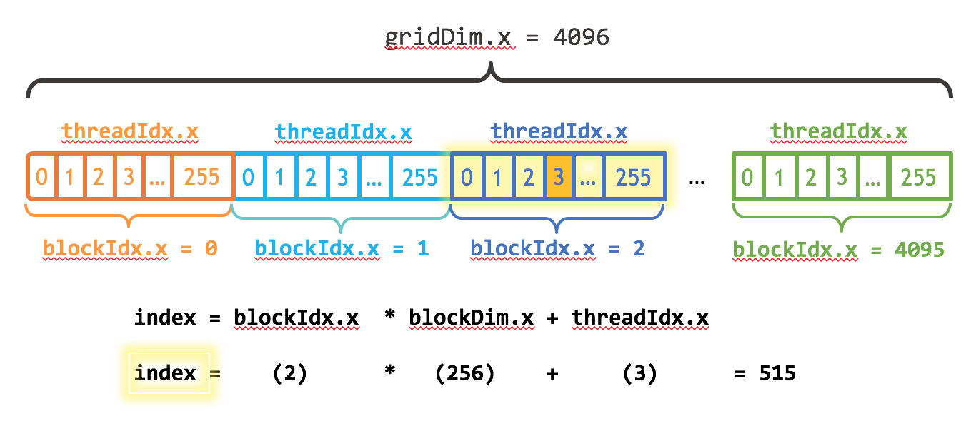
Now we get
Nvidia Quadro P1000: From 2.500 to 0.022 to 0.006 secs!
==10662== NVPROF is profiling process 10662, command: ./a.out
Max error: 0
==10662== Profiling application: ./a.out
==10662== Profiling result:
            Type  Time(%)      Time     Calls       Avg       Min       Max  Name
 GPU activities:  100.00%  6.0868ms         1  6.0868ms  6.0868ms  6.0868ms  add(int, float*, float*)
      API calls:   96.03%  165.28ms         2  82.641ms  13.911us  165.27ms  cudaMallocManaged
                    3.54%  6.0887ms         1  6.0887ms  6.0887ms  6.0887ms  cudaDeviceSynchronize
                    0.27%  460.56us         2  230.28us  184.71us  275.85us  cudaFree
                    0.13%  215.37us       101  2.1320us     133ns  151.55us  cuDeviceGetAttribute
                    0.02%  30.822us         1  30.822us  30.822us  30.822us  cudaLaunchKernel
                    0.01%  22.122us         1  22.122us  22.122us  22.122us  cuDeviceGetName
                    0.00%  5.7430us         1  5.7430us  5.7430us  5.7430us  cuDeviceGetPCIBusId
                    0.00%  1.3810us         3     460ns     203ns     945ns  cuDeviceGetCount
                    0.00%     921ns         2     460ns     163ns     758ns  cuDeviceGet
                    0.00%     438ns         1     438ns     438ns     438ns  cuDeviceTotalMem
                    0.00%     234ns         1     234ns     234ns     234ns  cuDeviceGetUuid

==10662== Unified Memory profiling result:
Device "Quadro P1000 (0)"
   Count  Avg Size  Min Size  Max Size  Total Size  Total Time  Name
      59  138.85KB  4.0000KB  0.9961MB  8.000000MB  740.3880us  Host To Device
      24  170.67KB  4.0000KB  0.9961MB  4.000000MB  337.8280us  Device To Host
      32         -         -         -           -  2.253582ms  Gpu page fault groups
Total CPU Page faults: 36
Testla T4: From 0.108 to 0.004 to 0.003 secs
==8972== NVPROF is profiling process 8972, command: ./cuda_04.x
Max error: 0
==8972== Profiling application: ./cuda_04.x
==8972== Profiling result:
            Type  Time(%)      Time     Calls       Avg       Min       Max  Name
 GPU activities:  100.00%  2.9741ms         1  2.9741ms  2.9741ms  2.9741ms  add(int, float*, float*)
      API calls:   98.47%  250.63ms         2  125.31ms  38.785us  250.59ms  cudaMallocManaged
                    1.18%  2.9959ms         1  2.9959ms  2.9959ms  2.9959ms  cudaDeviceSynchronize
                    0.24%  613.16us         2  306.58us  302.27us  310.89us  cudaFree
                    0.07%  188.26us       101  1.8630us     169ns  86.068us  cuDeviceGetAttribute
                    0.02%  38.874us         1  38.874us  38.874us  38.874us  cuDeviceGetName
                    0.01%  37.051us         1  37.051us  37.051us  37.051us  cudaLaunchKernel
                    0.00%  5.7050us         1  5.7050us  5.7050us  5.7050us  cuDeviceGetPCIBusId
                    0.00%  2.2980us         3     766ns     224ns  1.8050us  cuDeviceGetCount
                    0.00%     979ns         2     489ns     195ns     784ns  cuDeviceGet
                    0.00%     587ns         1     587ns     587ns     587ns  cuDeviceTotalMem
                    0.00%     367ns         1     367ns     367ns     367ns  cuModuleGetLoadingMode
                    0.00%     324ns         1     324ns     324ns     324ns  cuDeviceGetUuid

==8972== Unified Memory profiling result:
Device "Tesla T4 (0)"
   Count  Avg Size  Min Size  Max Size  Total Size  Total Time  Name
     106  77.282KB  4.0000KB  980.00KB  8.000000MB  969.6510us  Host To Device
      24  170.67KB  4.0000KB  0.9961MB  4.000000MB  363.6760us  Device To Host
      11         -         -         -           -  2.908132ms  Gpu page fault groups
Total CPU Page faults: 36
13.10.3. TODO Openmp offload to gpu
REF:
Code
#include <iostream>
#include <cstdio>
#include <omp.h>

int main()
{
    int a[100], b[100], c[100];
    int i;

    // Initialize arrays a and b
    for (i = 0; i < 100; i++) {
        a[i] = i;
        b[i] = 2 * i;
    }

    int num_devices = omp_get_num_devices();
    printf("Number of available devices %d\n", num_devices);

    // Offload computation to GPU
    #pragma omp target teams distribute parallel for map(to:a[0:100], b[0:100]) map(from:c[0:100])
    for (i = 0; i < 100; i++) {
        c[i] = a[i] + b[i];
    }

    // Print results
    for (i = 0; i < 100; i++) {
        std::cout << c[i] << " ";
    }
    std::cout << std::endl;

    return 0;
}
Does not work in sala2 due to the error
OpenMP GPU Offload is available only on systems with NVIDIA GPUs with compute capability '>= cc70
It seems that sala2 compute capability is 6.1. It can be get with
nvidia-smi --query-gpu=compute_cap --format=csv
Using google collab I can compile it
!nvcc -arch sm_75 -O3 -o openmp_offload openmp_offload.cpp -lgomp
and get
Number of available devices 1
0 3 6 9 12 15 18 21 24 27 30 33 36 ...
Check:
/* Copyright (c) 2019 CSC Training */
/* Copyright (c) 2021 ENCCS */
#include <stdio.h>

#ifdef _OPENMP
#include <omp.h>
#endif

int main()
{
  int num_devices = omp_get_num_devices();
  printf("Number of available devices %d\n", num_devices);

  #pragma omp target
  {
      if (omp_is_initial_device()) {
        printf("Running on host\n");
      } else {
        int nteams= omp_get_num_teams();
        int nthreads= omp_get_num_threads();
        printf("Running on device with %d teams in total and %d threads in each team\n",nteams,nthreads);
      }
  }
  return 0;
}
13.10.4. TODO OpenACC intro
REF:
- https://www.openacc.org/
- https://enccs.github.io/OpenACC-CUDA-beginners/1.02_openacc-introduction/
- https://ulhpc-tutorials.readthedocs.io/en/latest/gpu/openacc/basics/
Check if we are using the gpu or the cpu:
#include <stdio.h>
#include <openacc.h>

int main() {
  int device_type = acc_get_device_type();

  if (device_type == acc_device_nvidia) {
    printf("Running on an NVIDIA GPU\n");
  } else if (device_type == acc_device_radeon) {
    printf("Running on an AMD GPU\n");
    //} else if (device_type == acc_device_intel_mic) {
    //printf("Running on an Intel MIC\n");
  } else if (device_type == acc_device_host) {
    printf("Running on the host CPU\n");
  } else {
    printf("Unknown device type\n");
  }

  return 0;
}
Compile as
gcc -fopenacc mycode.c
Simple example:
#include <stdio.h>

int main() {
  int i;
  float a[100], b[100], c[100];

  // Initialize arrays
  for (i = 0; i < 100; i++) {
    a[i] = i;
    b[i] = i;
  }

  // Compute element-wise sum
  #pragma acc parallel loop
  for (i = 0; i < 100; i++) {
    c[i] = a[i] + b[i];
  }

  // Print result
  for (i = 0; i < 100; i++) {
    printf("%f\n", c[i]);
  }

  return 0;
}
14. Introduction to OpenMp (Shared memory)
This is an extension for languages like C/C++. It is targeted for multi-threaded, shared memory parallelism. It is very simple, you just add some pragma directives which, if not supported, are deactivated and then completely ignored. It is ideal for a machine with several cores, and shared memory. For much more info, see http://www.openmp.org/ and https://hpc-tutorials.llnl.gov/openmp/
14.1. Introduction: Hello world and threadid
Typical Hello world,
#include <cstdio>
#include "omp.h"

int main(void)
{
    double x = 9.0;
//#pragma omp parallel num_threads(4)
#pragma omp parallel
    {// se generan los threads
        std::printf("Hello, world.\n");
        std::printf("Hello, world2.\n");
    } // mueren los threads

    return 0;
}
This makes a parallel version if you compile with the -fopemp
flag. Test it. What happens if you write
export OMP_NUM_THREADS=8
and then you run the executable?
The actual directive is like
  #pragma omp parallel [clause ...]  newline
                     if (scalar_expression)
                     private (list)
                     shared (list)
                     default (shared | none)
                     firstprivate (list)
                     reduction (operator: list)
                     copyin (list)
                     num_threads (integer-expression)
   structured_block
But we will keep things simple.
What is really important to keep in mind is what variables are going to be shared and what are going to be private, to avoid errors, reca conditions, etc.
If you want to know the thread id, you can use
  int nth =  omp_get_num_threads();
  int tid =  omp_get_thread_num();
inside your code, as in the following,
#include <cstdio> // printf
#include <omp.h>

int main(void)
{
  double x = 9.0;

  int nth = omp_get_num_threads();
  int thid = omp_get_thread_num();
  std::printf("Hello world from thid: %d, out of %d .\n",
              thid, nth);

//#pragma omp parallel num_threads(4)
#pragma omp parallel
  {// se generan los threads
    int nth = omp_get_num_threads(); // al declarar aca, son privados
    int thid = omp_get_thread_num();
    std::printf("Hello world from thid: %d, out of %d .\n",
                thid, nth);
  } // mueren los threads

  std::printf("Hello world from thid: %d, out of %d .\n",
              thid, nth);


  return 0;
}
Please use the thread sanitize:
g++ -fopenmp -g -fsanitize=thread code.cpp
There are some other env variables that could be useful:
OMP_NUM_THREADS=4
OMP_DISPLAY_ENV=TRUE
OMP_DISPLAY_AFFINITY=TRUE
OMP_STACK_SIZE=1000000
14.2. Private and shared variables
Shared and private
#include <cstdio>
#include <omp.h>

int main(void)
{
  double x = 9.0;

  int nth = omp_get_num_threads();
  int thid = omp_get_thread_num();
  std::printf("Hello world from thid: %d, out of %d .\n",
              thid, nth);

//#pragma omp parallel num_threads(4)
#pragma omp parallel private(thid, nth)
  {// se generan los threads
    thid = omp_get_thread_num();
    nth = omp_get_num_threads();
    std::printf("Hello world from thid: %d, out of %d .\n",
                thid, nth);
  } // mueren los threads

  return 0;
}
#include <omp.h>
#include <stdio.h>

int main(int argc, char *argv[]) {

  int nthreads, tid;

  /* Fork a team of threads with each thread having a private tid variable */
#pragma omp parallel private(tid)
  {

    /* Obtain and print thread id */
    tid = omp_get_thread_num();
    printf("Hello World from thread = %d\n", tid);

    /* Only master thread does this */
    if (tid == 0)
    {
      nthreads = omp_get_num_threads();
      printf("Number of threads = %d\n", nthreads);
    }

  }  /* All threads join master thread and terminate */

}
In this example we see the memory address for shared and private variables to illustrate those concepts:
#include <omp.h>
#include <iostream>
#include <cstdio>

int main(int argc, char *argv[]) {

  int nthreads, tid;

  /* Fork a team of threads with each thread having a private tid variable */
#pragma omp parallel private(tid)
  {

    /* Obtain and print thread id */
    tid = omp_get_thread_num();
    std::printf("Hello World from thread = %d\n", tid);
    std::cout << "Memory address for tid = " << &tid << std::endl;
    std::cout << "Memory address for nthreads = " << &nthreads << std::endl;

    /* Only master thread does this */
    if (tid == 0)
      {
        nthreads = omp_get_num_threads();
        printf("Number of threads = %d\n", nthreads);
      }

  }  /* All threads join master thread and terminate */

  return 0;
}
14.3. Parallelizing a for loop
Condiciones del problema:
- Arreglo de tamanho N.
- Tenemos nth threads.
Nlocal = N/nthimin = tid*Nlocal, imax = (tid+1)*Nlocal = imin + Nlocal
14.3.1. Manually
The following code assigns the elements of a vector in parallel:
#include <omp.h>
#include <iostream>
#include <cmath>
#include <vector>
#include <cstdlib>
#include <numeric>

void fill(std::vector<double> & array);
double suma(const std::vector<double> & array);

int main(int argc, char *argv[])
{
  const int N = std::atoi(argv[1]);
  std::vector<double> data(N);

  // llenar el arreglo
  fill(data);
  //std::cout << data[0] << "\n";

  // calcular la suma y el promedio
  double total = suma(data);
  std::cout << total/data.size() << "\n";

  return 0;
}

void fill(std::vector<double> & array)
{
  int N = array.size();
#pragma omp parallel
  {
    int thid = omp_get_thread_num();
    int nth = omp_get_num_threads();
    int Nlocal = N/nth;
    int iimin = thid*Nlocal;
    int iimax = iimin + Nlocal;
    for(int ii = iimin; ii < iimax; ii++) {
      array[ii] = 2*ii*std::sin(std::sqrt(ii/56.7)) +
        std::cos(std::pow(1.0*ii*ii/N, 0.3));
    }
  }
}

double suma(const std::vector<double> & array)
{
  int N = array.size();
  std::vector<double> sumaparcial;
#pragma omp parallel
  {
    int thid = omp_get_thread_num();
    int nth = omp_get_num_threads();
    if (0 == thid) {
      sumaparcial.resize(nth);
    }
#pragma omp barrier
    double localsum = 0.0;
    int Nlocal = N/nth;
    int iimin = thid*Nlocal;
    int iimax = iimin + Nlocal;
    for(int ii = iimin; ii < iimax; ii++) {
      localsum += array[ii];
    }
    sumaparcial[thid] = localsum;
  }
  return std::accumulate(sumaparcial.begin(), sumaparcial.end(), 0.0);
}
OLD
#include <omp.h>
#include <iostream>
#include <cmath>
#include <vector>

int main(int argc, char *argv[]) {

  const int N = 80000000;
  int i;
  double *a = new double[N];

#pragma omp parallel private(i)
  {
    int thid = omp_get_thread_num();
    int nth = omp_get_num_threads();
    int localsize = N/nth;
    int iimin = thid*localsize;
    int iimax = iimin + localsize;
    for(i = iimin; i < iimax; i++) {
      a[i] = 2*i*std::sin(std::sqrt(i/56.7)) +
        std::cos(std::pow(i*i, 0.3));
    }
  }

  std::cout << a[1] << "\n";

  delete [] a;
  return 0;
}
14.3.2. Using omp parallel for
#include <omp.h>
#include <iostream>
#include <cmath>
#include <vector>
#include <cstdlib>
#include <numeric>

void fill(std::vector<double> & array);
double suma(const std::vector<double> & array);

int main(int argc, char *argv[])
{
  const int N = std::atoi(argv[1]);
  std::vector<double> data(N);

  // llenar el arreglo
  fill(data);
  //std::cout << data[0] << "\n";

  // calcular la suma y el promedio
  double total = suma(data);
  std::cout << total/data.size() << "\n";

  return 0;
}

void fill(std::vector<double> & array)
{
  const int N = array.size();
#pragma omp parallel for
  for(int ii = 0; ii < N; ii++) {
      array[ii] = 2*ii*std::sin(std::sqrt(ii/56.7)) +
        std::cos(std::pow(1.0*ii*ii/N, 0.3));
  }
}

double suma(const std::vector<double> & array)
{
  int N = array.size();
  double suma = 0.0;
#pragma omp parallel for reduction(+:suma)
  for(int ii = 0; ii < N; ii++) {
    suma += array[ii];
  }
  return suma;
}
OLD
#include <omp.h>
#include <iostream>
#include <cmath>

void fill(double * array, int size);
double average(double * array, int size);

int main(int argc, char *argv[]) {
  const int N = std::atoi(argv[1]);
  double *a = new double[N];

  fill(a, N);
  std::cout << a[1] << "\n";

  //std::cout << average(a, N) << "\n";

  double suma = 0.0;
#pragma omp parallel for reduction(+:suma)
  for(int i = 0; i < N; i++) {
    suma += a[i];
  }
  std::cout <<  suma/N << "\n";

  delete [] a;
  return 0;
}

void fill(double * array, int size)
{
#pragma omp parallel for
  for(int i = 0; i < size; i++) {
    array[i] = 2*i*std::sin(std::sqrt(i/56.7)) +
      std::cos(std::pow(1.0*i*i, 0.3));
  }
}
double average(double * array, int size)
{
  double suma = 0.0;
#pragma omp parallel for reduction(+:suma)
  for(int i = 0; i < size; i++) {
    suma += array[i];
  }
  return suma/size;
}
Exercise: Modify the code to be able to compute the mean in parallel. Play with larger and larger arrays and also with increasing the number of processors. Can you compute any parallel metric?
#include <omp.h>
#include <iostream>
#include <cmath>

void fill_data(double *a, int size);
double average(double *a, int size);

int main(int argc, char *argv[]) {
    std::cout.precision(15); std::cout.setf(std::ios::scientific);

    const int N = 80000000;
    int i;
    double *a = new double[N];

    fill_data(a, N);
    std::cout << a[1] << std::endl;
    double avg = average(a, N);
    std::cout << avg << "\n";

    delete [] a;
    return 0;
}

void fill_data(double *a, int size)
{
    long int i;
#pragma omp parallel for
    for(i = 0; i < size; i++) {
        a[i] = 2*i*std::sin(std::sqrt(i/56.7)) +
            std::cos(std::pow(i*i, 0.3));
    }
}

double average(double *a, int size)
{
    double result = 0;
#pragma omp parallel for reduction(+:result)
    for(int ii = 0; ii < size; ++ii) {
      result = result + a[ii];
    }
    result /= size;
    return result;
}
14.3.3. Using reductions
This example shows how to reduce a variable using the reduction keyword:
  #include <iostream>
#include <cmath>

int main(int argc, char ** argv)
{
  const int N = 100000000;
  int i;
  double *a;
  a = new double [N];
  double suma = 0;

#pragma omp parallel for reduction(+:suma)
  for (i = 0; i < N; ++i) {
    a[i] = 2*std::sin(i/35.6);
    suma += a[i];
  }

  std::cout << suma << std::endl;

  delete [] a;
  return 0;
}
Now read the following code, try to predict its outcome, and then run it and test your prediction (from https://computing.llnl.gov/tutorials/openMP/#Introduction) :
    #include <omp.h>
    #define N 1000
    #define CHUNKSIZE 100

    main(int argc, char *argv[]) {

      int i, chunk;
      float a[N], b[N], c[N];

      /* Some initializations */
      for (i=0; i < N; i++)
        a[i] = b[i] = i * 1.0;
      chunk = CHUNKSIZE;

    #pragma omp parallel shared(a,b,c,chunk) private(i)
      {

    #pragma omp for schedule(dynamic,chunk) nowait
        for (i=0; i < N; i++)
    c[i] = a[i] + b[i];

      }   /* end of parallel region */
      return 0;
    }
14.4. Exercises
Refs: CT-LAB openmp exercises; https://computing.llnl.gov/tutorials/openMP/exercise.html
Write a program to compute the mean and the standard deviation for a large array using OpenMP, with only one reduction. Also compute the parallel metrics.
// stats.cpp
#include <omp.h>
#include <iostream>
#include <cmath>
#include <vector>
#include <cstdlib>
#include <numeric>

void fill(std::vector<double> & array);
void stats(const std::vector<double> & array, double &mean, double &sigma);

int main(int argc, char *argv[])
{
  const int N = std::atoi(argv[1]);
  std::vector<double> data(N);

  // llenar el arreglo
  fill(data);

  // calcular stats
  double mean{0.0}, sigma{0.0};
  double start = omp_get_wtime();
  stats(data, mean, sigma);
  double time = omp_get_wtime() - start;
  std::printf("%.15le\t\t%.15le\t\t%.15le\n", mean, sigma, time);

  return 0;
}

void fill(std::vector<double> & array)
{
  const int N = array.size();
#pragma omp parallel for
  for(int ii = 0; ii < N; ii++) {
      array[ii] = 2*ii*std::sin(std::sqrt(ii/56.7)) +
        std::cos(std::pow(1.0*ii*ii/N, 0.3));
  }
}

void stats(const std::vector<double> & array, double & mean, double & sigma)
{
  int N = array.size();
  double suma = 0.0;
#pragma omp parallel for reduction(+:suma)
  for(int ii = 0; ii < N; ii++) {
    suma += array[ii];
  }
  mean = suma/N;
}
Write a program to compute the integral of the function \(y = x^{2}\), for $ x ∈ [0, 10]$. Fill the following table:
# Threads Runtime [s] Speedup Efficiency Explain your results in terms of the number of processors available. Use \(N=12000\). Do it in two ways:
- Distributing the N intervals across all threads, so each one has a smaller part.
- Keeping constant the resolution per thread, that is , each trhead has N intervals.
What is the difference between the two cases, regarding the precision and the time?
    #include <iostream>
    #include <omp.h>

    using fptr = double(double);

    double f(double x);
    double integral_serial(double a, double b, int N, fptr f);
    double integral_openmp(double a, double b, int N, fptr f);

    int main(void)
    {
      // declare vars
      const double XA = 0.0;
      const double XB = 10.0;
      const int N = 100000000;

      // print result
      //std::cout << "Serial integral: " << integral_serial(XA, XB, N, f) << "\n";
      //std::cout << "Serial openmp  : " << integral_openmp(XA, XB, N, f) << "\n";
      double t1 = omp_get_wtime();
      integral_openmp(XA, XB, N, f);
      double t2 = omp_get_wtime();

    #pragma omp parallel
      {
        if(0 == omp_get_thread_num()) {
          std::cout << omp_get_num_threads() << "\t" << t2 - t1 << std::endl;
        }
      }
    }

    double f(double x)
    {
      return x*x;
    }

    double integral_serial(double a, double b, int N, fptr f)
    {
      const double dx = (b-a)/N;
      // compute integral
      double sum = 0, x;
      for(int ii = 0; ii < N; ++ii) {
        x = a + ii*dx;
        sum += dx*f(x);
      }
      return sum;
    }

    double integral_openmp(double a, double b, int N, fptr f)
    {
      TODO
    }
- Parallelize a Matrix-Matrix multiplication. Compare the performance when you use one, two, three, for threads.
Is this loop parallelizable? If not, why?
 #pragma omp parallel for
 for (int i = 1; i < N; i++)
 {
   A[i] = B[i] – A[i – 1];
 }
- Parallelize a matrix-vector multiplication. What must be shared? what should be private?
- Parallelize the matrix transposition.
- Check and solve the exercises on https://computing.llnl.gov/tutorials/openMP/exercise.html .
- Check and solve http://www.hpc.cineca.it/content/training-openmp .
- Some other examples are at https://www.archer.ac.uk/training/course-material/2015/03/thread_prog/ .
15. Introduction to MPI (distributed memory)
15.1. Intro MPI
MPI stands for Message Passing Interface. It is a standard which allows processes to communicate and share data across an heterogeneous setup. MPI is well suited for distributed memory systems, although it can also be used in multiprocessor environments (on those environments, OpenMP is a better suited solution). Both MPI (on any of its implementations) and OpenMP represent the most common approaches to program on a cluster environment.
NOTE: This section is heavily based on Chapter 13 of “High Performance Linux Clusters with Oscar, Rocks, OpenMosix, and MPI”, J. D. Sloan, O’Reilly.
MPI is a library of routines which allows the parts of your parallel program to communicate. But it is up to you how to split up your program/problem. There are no typical restrictions on the number of processors you can split on your problem: you can use less or more process than the number of available processors. For that reason, MPI allows you to tag every process with a given rank, on a problem of size total number of processes.
MPI can be used as a library on several languages: Fortran, C, C++ , etc. In the following, we will use mostly C.
15.2. Core MPI
It is typical to denote the rank-0 process as the master and the remaining process (rank >= 1) as slaves. Most of the time, the slaves are processing several parts of the problem and then communicate back the results to the master. All of this is managed on a single source code which is advantageous. The following is an example of the most fundamental MPI program which constitutes a template for more complex programs:
  #include "mpi.h"
  #include <cstdio>

  int main(int argc, char **argv)
  {
    int processId;                 /* rank of process */
    int noProcesses;               /* number of processes */

    MPI_Init(&argc, &argv);                   /* Mandatory */
    MPI_Comm_size(MPI_COMM_WORLD, &noProcesses);
    MPI_Comm_rank(MPI_COMM_WORLD, &processId);

    std::fprintf(stdout, "Hello from process %d of %d\n", processId, noProcesses);

    MPI_Finalize();                       /* Mandatory */

    return 0;
  }
Before compiling and running, we will explain the code. First of all,
the MPI functions are added by the inclusion of the mpi.h header. The
two mandatory functions MPI_Init and MPI_Finalize, must be always
present. They set-up and destroy the MPI running environment. The other
two, MPI_Comm_size and MPI_Comm_rank allows to identify the size of
the problem (number of processes) and the rank of the current process.
This allows to distinguish the master from the slaves and to split the
problem.
- MPIInit
- This function call must occur before any other MPI function call. This function initializes the MPI session. It receives the argc and argv arguments, as shown, which allows the program to read command line arguments.
- MPIFinalize
- This function releases the MPI environment. This should be the last call to MPI in the program, after all communications have ended. Your code must be written in such a way that all processes call this function.
- MPICommsize
- This function returns the total number of processes
running on a communicator. A communicator is the communication group
used by the processes. The default communicator is
MPI_COMM_WORLD. You can create your own communicators to isolate several sub-groups of processes. - MPICommrank
- Returns the actual rank of the calling process, inside the communicator group. The range goes from 0 to the the size minus 1.
15.2.1. MPIGetprocessorname
This retrieves the hostname of the current and is very useful for debugging purposes. The following example shows how to get the node name
  #include "mpi.h"
  #include <cstdio>

  int main(int argc, char **argv)
  {
    int processId;                 /* rank of process */
    int noProcesses;               /* number of processes */
    int nameSize;              /* lenght of name */
    char computerName[MPI_MAX_PROCESSOR_NAME];

    MPI_Init(&argc, &argv);                   /* Mandatory */
    MPI_Comm_size(MPI_COMM_WORLD, &noProcesses);
    MPI_Comm_rank(MPI_COMM_WORLD, &processId);

    MPI_Get_processor_name(computerName, &nameSize);
    fprintf(stderr, "Hello from process %d of %d, on %s\n", processId, noProcesses, computerName);

    MPI_Finalize();                       /* Mandatory */

    return 0;
  }
15.2.2. Compiling and running the MPI program
Compilation can be done directly with the gcc compiler by using the
appropriate flags. But there is a helper command ready to help you:
mpicc. Save the previous example code into a file (here called
mpi-V1.c) and run the following command
$ mpicc mpi-V1.c -o hello.x
If you run the command as usual, it will expand to the number of local cores and run locally only (for example, ina two cores system):
     $ ./hello.x
     Hello from process 0 of 2, on iluvatarMacBookPro.local
     Hello from process 1 of 2, on iluvatarMacBookPro.local
But, there is another utility which allows you to specify several parameters, like the number of processes to span, among others:
     $ mpirun -np 5 ./hello.x
     Hello from process 3 of 5, on iluvatarMacBookPro.local
     Hello from process 1 of 5, on iluvatarMacBookPro.local
     Hello from process 4 of 5, on iluvatarMacBookPro.local
     Hello from process 0 of 5, on iluvatarMacBookPro.local
     Hello from process 2 of 5, on iluvatarMacBookPro.local
15.2.3. Running an mpi on several machines
You can run an mpi process on the same machine or in several machines, as follows
$ mpirun -np 4 -host host01,host02 ./a.out
where host01, etc is the hostname where you want to run the process. You will
need to have access by ssh to those hosts, and preferable, a password-less setup
. See also the manual for mpirun .
You can specify a machine file for mpi tu use them and run the command with given resources. An example machine files is as follows
      hostname1 slots=2
      hostname2 slots=4
      hostname3 slots=6
where hostname is the ip or the hostname of a given machine and the slots indicates how many jobs to run. You will need to have a passwordless access or similar to those computers.
To configure the passwordless ssh, you can follow the many tutorials online, which basically are the following steps
Generate the rsa key
ssh-keygen -t rsa
Do not set ay passphrase, just press enter.
Copy the id to the computer where you want to run processes remotely,
ssh-copy-id 192.168.10.16
Enter your password for the last time. If everything goes ok, test that you can login remotely without password by runnung
ssh 192.168.10.16
Now you can run the process remotely:
mpirun -np 100 -host 192.168.10.15,192.168.10.16 --oversubscribe ./a.out
15.3. Application: Numerical Integration (Send and Recv functions)
To improve our understanding of MPI, and to introduce new functions, we will use a familiar problem to investigate: the computation of the area under a curve. Its easiness and familiarity allows to focus on MPI and its usage. Let’s introduce first the serial version.
15.3.1. Serial implementation of the numerical integration by rectangles
#include <cstdio>

/* Problem parameters */
double f(double x);
double integral_serial(double xmin, double xmax, double n);

int main(int argc, char **argv)
{
  const int numberRects = 50;
  const double lowerLimit = 2.0;
  const double upperLimit = 5.0;

  double integral = integral_serial(lowerLimit, upperLimit, numberRects);
  printf("The area from %lf to %lf is : %lf\n", lowerLimit, upperLimit, integral);

  return 0;
}

double f(double x) {
  return x*x;
}

double integral_serial(double xmin, double xmax, double n)
{
  double area = 0.0;
  double width = (xmax - xmin)/n;

  for (int i = 0; i < n; ++i) {
    double at = xmin + i*width + width/2.0; // center in the middle
    double heigth = f(at);
    area = area + width*heigth;
  }
  return area;
}
Compile and run it :
$ g++ serial_integral.cpp
$ ./a.out
The area from 2.000000 to 5.000000 is : 38.999100
Now let’s implement an mpi solution.
15.3.2. MPI solution: Point to point communication with MPISend and MPIRecv
Check: https://mpitutorial.com/tutorials/mpi-send-and-receive/
This is an embarrassingly parallel problem. There are no data dependencies. We
can partition the domain, performing partial sums per process, and then cumulate
all of them. Basically, we will use MPI_Comm_rank and MPI_Comm_size to
partition the problem, and we will introduce two new functions: MPI_Send, to
send data, and MPI_Recv, to receive data. These are known as blocking,
point-to-point communications.
Before checking the code, please work in groups to deduce the right problem partition (keeping the same number of inteervals per process) and how to communicate data. Use a shared whiteboard, like google jamboard.
#include "mpi.h"
#include <cstdio>
#include <cstdlib>

/* Problem parameters */
double f(double x);
double integral_serial(double xmin, double xmax, double n);
void integral_mpi(double xmin, double xmax, double n, int pid, int np);

int main(int argc, char **argv)
{
  const int numberRects = std::atoi(argv[1]);
  const double lowerLimit = 2.0;
  const double upperLimit = 5.0;

  /* MPI Variables */

  /* problem variables */
  int pid, np;

  /* MPI setup */
  MPI_Init(&argc, &argv);
  MPI_Comm_size(MPI_COMM_WORLD, &np);
  MPI_Comm_rank(MPI_COMM_WORLD, &pid);

  integral_mpi(lowerLimit, upperLimit, numberRects, pid, np);

  /* finish */
  MPI_Finalize();

  return 0;
}

double integral_serial(double xmin, double xmax, double n)
{
  double area = 0.0;
  double width = (xmax - xmin)/n;

  for (int i = 0; i < n; ++i) {
    double at = xmin + i*width + width/2.0; // center in the middle
    double heigth = f(at);
    area = area + width*heigth;
  }
  return area;
}

void integral_mpi(double xmin, double xmax, double n, int pid, int np)
{
  /* Adjust problem size for sub-process */
  double range = (xmax - xmin) / np;
  double lower = xmin + range*pid;

  /* Calculate area for subproblem */
  double area = integral_serial(lower, lower+range, n);

  /* Collect info and print results */
  MPI_Status status;
  int tag = 0;
  if (0 == pid) { /* Master */
    double total = area;
    for (int src = 1; src < np; ++src) {
      MPI_Recv(&area, 1, MPI_DOUBLE, src, tag, MPI_COMM_WORLD, &status);
      total += area;
    }
    fprintf(stderr, "The area from %g to %g is : %25.16e\n", xmin, xmax, total);
  }
  else { /* slaves only send */
    int dest = 0;
    MPI_Send(&area, 1, MPI_DOUBLE, dest, tag, MPI_COMM_WORLD);
  }
}


double f(double x) {
  return x*x;
}
Compile as usual,
mpic++ mpi_integral.cpp
and run it
$ mpirun -np 2 ./a.out
$ mpirun -np 10 ./a.out
Exercise: Play with the number of processes. Are you getting a better answer for increasing number of processes?
In this example we have kept constant the number of rectangles per range. That means that as the number of processess increases, the total number of rectangles increases too, since each process has the same original number of rectangles. Therefore, the more the processes, the better the precision. If you prefer speed over precision, you will have to fix the total number of rectangles, whose number per processor will decrease.
Exercise : Change the previous code to handle a constant number of rectangles. As you increase the number of processors, is the precision increasing? or the speed?
The important part here is the scaling of the problem to the actual number of processes. For example, for five processes, we need first to divide the total interval (from 2 to 5 in tis example) into the number of processes, and then take each one of this sub-intervals and process it on the given process (identified by processId). This is called a domain-decomposition approach.
At the end of the code, we verify if we are on a slave or on the master. If we
are the master, we receive all the partial integrations sent by the slaves, and
then we print the total. If we are a slave, we just send our result back to the
master (destination = 0). Using these functions is simple but not always
efficient since, for example, for 100 processes, we are calling MPI_Send and
MPI_Recv 99 times.
MPI_Send- used to send information to one process to another. A call to
MPI_SendMUST be matched with a correspondingMPI_Recv. Information is typed (the type is explicitly stated), and tagged. The first argument ofMPI_Sendgives the starting address of the data to be transmitted. The second is the number of items to be sent, and the third one is the data type (MPI_DOUBLE). There are more datatypes likeMPI_BYTE,MPI_CHAR,MPI_UNSIGNED,MPI_INT,MPI_FLOAT,MPI_PACKED, etc. The next argument is the destination, that is, the rank of the receiver. The next one is a tag, which is used for buffer purposes. Finally, the (default) communicator is used. MPI_Recv- allows to receive information sent by
MPI_Send. Its first three arguments are as before. Then it comes the destination (rank of the receiving process), the tag, the communicator, and a status flag.
Both MPI_Send and MPI_Recv are blocking calls. If a process is receiving
information which has not been sent yet, if waits until it receives that info
without doing anything else.
Before continue, please check the following mpi functions:
MPI_ISend , MPI_IrecvMPI_SendrecvMPI_Sendrecv_replace
Exercise: Discuss if any of the previous can be used for the integral. Or what pattern would you think could be useful? maybe a reduction?
15.4. More Point to point exercises
Check also: http://www.archer.ac.uk/training/course-material/2017/09/mpi-york/exercises/MPP-exercises.pdf
15.4.1. Ping-Pong
Ref: Gavin, EPCC • Write an MPI code for 2 processes • The first task sends a message to the second task • The message can be a single integer • The second task receives this message • The second task changes the message somehow
- Add 99 to the original message, for instance
• The second task sends the message back to the first task
- The first task receives the message
• The first task prints this new message to the screen Maybe repeat M times
15.4.2. Bandwitdh local and network
Compute the bandwidth when sending data locally (same computer) and to other computer in the network. Plot the time taken to send the data as a function of the buffer size. Is the bandwidth (Mbits/s) constant? is there any difference between local and multimachine data sending?
15.4.3. Large unit matrix
Imagine a large unit matrix that is distributed among all the processes in horizontal layers. Each process stores only its corresponding matrix part, not the full matrix. Make each process fill its corresponding part and then print the full matrix in the right order in the master process by sending each process matrix section to the master. Also plot it in gnupot or matplotlib
15.4.4. Ring pattern
Ref: Gavin, EPCC
- Write an MPI code which sends a message around a ring
- Each MPI task receives from the left and passes that message on to the right
- Every MPI task sends a message: Its own rank ID
- How many steps are required for the message to return ‘home’.
- Update the code so that each MPI Tasks takes the incoming message (an integer), and adds it to a running total
- What should the answer be on MPI Task 0 . Is the answer the same on all tasks? (Test with unblocking send and even/odd send receive)
15.5. Collective Communications
Check: https://mpitutorial.com/tutorials/mpi-broadcast-and-collective-communication/
If you check some of the previous code, or the integral code, we are sending the
same info over and over to every other process. While the master sends the data
to process 1, the remaining processes are idle. This is not efficient.
Fortunately, MPI provides several functions to improve this situation, where the
overall communication is managed much better. The first function is MPI_Bcast.
- MPIBcast
- provides a mechanism to distribute the same information
among a communicator group, in an efficient manner. It takes five arguments. The first three are the data to be transmitted, as usual. The fourth one is the rank of the process generating the broadcast, a.k.a the root of the broadcast. The final argument is the communicator identifier. See: https://www.open-mpi.org/doc/v4.1/man3/MPI_Bcast.3.php . The syntax is
int MPI_Bcast(void *buffer, int count, MPI_Datatype datatype,
              int root, MPI_Comm comm)
where root is the one sending the data in buffer to all other processes.

It could be internally optimized to reduce calls

- MPIReduce
- allows to collect data and, at the same time, perform a
mathematical operation on it (like collecting the partial results and then
summing up them). It requires not only a place where to put the results but also
the operator to be applied. This could be, for example, MPI_SUM, MPI_MIN,
MPI_MAX, etc. It also needs the identifier of the root of the broadcast. Both
this functions will simplify a lot the code, and also make it more efficient
(since the data distribution and gathering is optimised).
https://mpitutorial.com/tutorials/mpi-reduce-and-allreduce/

Check: https://mpitutorial.com/tutorials/mpi-broadcast-and-collective-communication/ http://wgropp.cs.illinois.edu/courses/cs598-s15/lectures/lecture29.pdf
15.5.1. MPI Bcast
- Sending an array from one source to all processes
#include "mpi.h"
#include <iostream>
#include <cstdlib>
#include <algorithm>
#include <numeric>

void send_data_collective(int size, int pid, int np);

int main(int argc, char **argv)
{
  int np, pid;

  /* MPI setup */
  MPI_Init(&argc, &argv);
  MPI_Comm_size(MPI_COMM_WORLD, &np);
  MPI_Comm_rank(MPI_COMM_WORLD, &pid);

  const int SIZE = std::atoi(argv[1]);
  send_data_collective(SIZE, pid, np);

  MPI_Finalize();

  return 0;
}

void send_data_collective(int size, int pid, int np)
{
  // create data buffer (all processes)
  double * data = new double [size];
  if (0 == pid) {
    std::iota(data, data+size, 0.0); // llena como 0 1 2 3 4
  }
  // send data to all processes
  int root = 0;
  double start = MPI_Wtime();
  MPI_Bcast(&data[0], size, MPI_DOUBLE, root, MPI_COMM_WORLD);
  double end = MPI_Wtime();
  // print size, time, bw in root
  if (0 == pid) {
    int datasize = sizeof(double)*size;
    std::cout << datasize << "\t" << (end-start) << "\t"
              << datasize/(end-start)/1.0e6 << "\n";
  }
  delete [] data;
}
- [Minihomework] Mesuring the bandwidth and comparing with simple send and recv
#include "mpi.h"
#include <iostream>
#include <cstdlib>
#include <algorithm>
#include <numeric>

void send_data_collective(int size, int pid, int np);
void send_data_point_to_point(int size, int pid, int np);

int main(int argc, char **argv)
{
  int np, pid;

  /* MPI setup */
  MPI_Init(&argc, &argv);
  MPI_Comm_size(MPI_COMM_WORLD, &np);
  MPI_Comm_rank(MPI_COMM_WORLD, &pid);

  const int SIZE = std::atoi(argv[1]);
  send_data_collective(SIZE, pid, np);

  MPI_Finalize();

  return 0;
}

void send_data_point_to_point(int size, int pid, int np)
{
// ???
}

void send_data_collective(int size, int pid, int np)
{
  // create data buffer (all processes)
  double * data = new double [size];
  std::iota(data, data+size, 0.0);
  // send data to all processes
  int root = 0;
  double start = MPI_Wtime();
  MPI_Bcast(&data[0], size, MPI_DOUBLE, root, MPI_COMM_WORLD);
  double end = MPI_Wtime();
  // print size, time, bw in root
  if (0 == pid) {
    int datasize = sizeof(double)*size;
    std::cout << datasize << "\t" << (end-start) << "\t"
              << datasize/(end-start)/1.0e6 << "\n";
  }
  delete [] data;
}
15.5.2. MPIBcast, MPIReduce
In this case we will read some data in process 0 , then broadcast it to other processes, and finally reduce back some result (an integral , in this example).
#include "mpi.h"
#include <cstdio>

/* Problem parameters */
double f(double x);

int main(int argc, char **argv)
{
  /* MPI Variables */
  int dest, noProcesses, processId, src, tag;
  MPI_Status status;

  /* problem variables */
  int i;
  double area, at, heigth, width, total, range, lower;
  int numberRects;
  double lowerLimit;
  double upperLimit;


  /* MPI setup */
  MPI_Init(&argc, &argv);
  MPI_Comm_size(MPI_COMM_WORLD, &noProcesses);
  MPI_Comm_rank(MPI_COMM_WORLD, &processId);

  /* read, send, and receive parameters */
  tag = 0;
  if (0 == processId) {
    fprintf(stderr, "Enter number of steps: \n");
    scanf("%d", &numberRects);
    fprintf(stderr, "Enter lower limit: \n");
    scanf("%lf", &lowerLimit);
    fprintf(stderr, "Enter upper limit: \n");
    scanf("%lf", &upperLimit);
  }

  /* Broadcast the read data parameters*/
  MPI_Bcast(&numberRects, 1, MPI_INT,    0, MPI_COMM_WORLD);
  MPI_Bcast(&lowerLimit,  1, MPI_DOUBLE, 0, MPI_COMM_WORLD);
  MPI_Bcast(&upperLimit,  1, MPI_DOUBLE, 0, MPI_COMM_WORLD);

  /* Adjust problem size for sub-process */
  range = (upperLimit - lowerLimit) / noProcesses;
  width = range / numberRects;
  lower = lowerLimit + range*processId;

  /* Calculate area for subproblem */
  area = 0.0;
  for (i = 0; i < numberRects; ++i) {
    at = lower + i*width + width/2.0;
    heigth = f(at);
    area = area + width*heigth;
  }

  /* Collect and reduce data */
  MPI_Reduce(&area, &total, 1, MPI_DOUBLE, MPI_SUM, 0, MPI_COMM_WORLD);

  /* print results */
  if (0 == processId) { /* Master */
    std::fprintf(stderr, "The area from %g to %g is : %25.16e\n", lowerLimit, upperLimit, total);
  }

  /* finish */
  MPI_Finalize();

  return 0;
}

double f(double x) {
  return x*x;
}
The eight functions MPI_Init, MPI_Comm_size, MPI_Comm_rank,
MPI_Send, MPI_Recv, MPI_Bcast, MPI_Reduce, and MPI_Finalize
are the core of the MPI programming. You are now and MPI programmer.
15.5.3. Exercises
- Modularize the previous integral code with functions. Basically use the same code as with send/recv but adapt it to use bcast/reduce.
- Do the same for the problem of computing the L2 norm (Euclidean norm) of a very large vector. Fill it with ones and test the answer. What kind of cpu time scaling do you get as function of the number of processes, with N = 100000?
- Filling randomly a matrix with probability \(p\): Make process 0 send the value of \(p\) to all processes. Also, distribute the matrix (only one slice per process). Fill the matrix at each process with prob \(p\). To verify, compute, at each process, the total places filled and send it to process 0. Add up all of them and print (from process 0) both the total proportion of filled sites (must be close to \(p\)) and the full matrix. Think if the algorithm that you devised to detect percolant clusters can be parallelized.
15.6. More examples : MPI_Gather, MPI_Scatter
Check:
- https://mpitutorial.com/tutorials/mpi-scatter-gather-and-allgather/
- http://wgropp.cs.illinois.edu/courses/cs598-s15/lectures/lecture29.pdf
- https://en.wikipedia.org/wiki/Collective_operation
Functions :
MPI_Scatter:Sends parts of a given data to corresponding processes. Example: Array 16 doubles. You have 4 processes. Then this functions sends the first 4 doubles to rank 0, the second 4 doubles to rank 1, and so on. Note: The original array must exists on the sending process, so this might limit its size.MPI_Gather:It is the opposite. Recovers data from all processes and stores it on the root process.
Now let’s do some a program to practice them. This program will compute the average of a set of random numbers. We will try not to share the full array of random numbers, but instead to make each process create its own array. We will use a Gaussian random number generator with mean 1.23 and sigma 0.45:
- Share with all processes the local array size (
N/np, whereNis the array size andnpis the number of processes), the mean and the sigma. - Share with all process the seed for the local random number generator. The seed might be the rank. Store the seeds on a local array and then send them from rank 0.
- Compute the local sum on each process.
- Get the local sum by storing it on the seeds array (for now, don’t reduce).
- Compute the mean and print it.
There are many other collective communications functions worth mentioning (https://en.wikipedia.org/wiki/Collective_operation , https://www.mpi-forum.org/docs/mpi-1.1/mpi-11-html/node64.html, https://www.rookiehpc.com/mpi/docs/index.php ):
- MPIScatter and MPIGather
- MPIAllGather and MPIAlltoall
- MPIScatterv
- MPIReduce, MPIScan, MPIExScan, ReduceScatter
Exercise: Each group will implement a working example of each of the following functions, as follows: https://www.rookiehpc.com/mpi/docs/index.php
| Group | Example |
|---|---|
| 1 | MPIscatter and MPIGather, MPIallgather |
| 2 | MPIScatterv, MPIGatherv |
| 3 | MPIAlltoall, MPIalltoallv |
| 4 | MPIReduce, MPIReducescatter |
| 5 | MPIScan, MPIExscan |
| 6 | MPIAll`Reduce with many MPIOP (min, max, sum , mult) |
15.7. Collective comms exercises
- Revisit all point-to-point comms exercises and implement them using collective comms if possible.
- Ring code
REF: Gavin, EPCC
- Use a Collective Communications routine to produce the same result as your Ring Code so that only Task 0 ‘knows’ the answer.
- Now change the Collective Communications call so all tasks ‘know’ the answer.
- Can you think of another way to implement the collective communications routine than the Ring Code?
- Compare the execution times for both the Ring Code and the associated Collective Communication routine.
- Which is faster?
- Why do the times change so much when you run it again and again?
- What happens when the size of the message goes from 1 MPIINT to 10000 MPIINTs?!
- Scaling for mpi integral Compute the scaling of the mpi integral code when using point to point and collective communications, in the same machine. Then do the same for two machines, dividing the number of processes among them.
- You will compute the polynomial \(f(x) = x + x^{2} + x^{3} + x^{4} + \ldots + x^{N}\). Write an mpi program that computes this in \(N\) processes and prints the final value on master (id = 0) for \(x = 0.987654\) and \(N = 25\). Use broadcast communications when possible.
- Compute the mean of a large array by distributing it on several processes. Your program must print the partial sums on each node and the final mean on master.
- Compute the value of \(\pi\) by using the montecarlo method: Imagine a circle of radius 1. Its area would be \(\pi\). Imagine now the circle inscribed inside a square of length 2. Now compute the area (\(\pi\)) of the circle by using a simple Monte-Carlo procedure: just throw some random points inside the square (\(N_s\)) and count the number of points that fall inside the circle (\(N_c\)). The ratio of the areas is related with the ratio of inner points as \(A_c/A_s \simeq N_c/N_s\), therefore \(A_C \simeq A_s N_c/N_s\). Use as many processes as possible to increase the precision. At the end print the total number of points tested, the value of \(\pi\) found, and the percent difference with the expected value, \(\Delta\). Plot \(\Delta\) as function of \(N_p\).
15.8. Practical example: Parallel Relaxation method
In this example we will parallelize the relaxation method by using MPI. We will decompose the domain, add some ghost zones and finally transmit some information between different processors. Our tasks will be as follows:
- Probar la version serial.
- Por cada proceso, crear el arreglo local incluyendo los ghosts: Probar llenando esta matriz con el pid y luego imprimir la matriz completa incluyendo y sin incluir los ghost (inicialización)
- Paralelizar la inicializacion e imprimir comparando con la version serial.
- Paralelizar las condiciones de frontera
- Comunicacion entre procesos: Enviar y recibir de vecinos y guardar en las zonas ghost. Imprimir para verificar. Introducir y probar diversas formas de comunicación, como Send y Recv, llamadas no bloqueantes, Sendrecv, y MPINeighborªlltoallw con MPICreatecart.
- Paralelizar la evolucion. Tener en cuenta las condiciones de frontera.
- Medir metricas paralelas y medir el tiempo de comunicacion.
- Extender a codiciones de frontera internas Usar un arreglo booleano que indique si una celda es frintera
- Calcular tambien el campo y/o densidades de carga.
To decompose the domain, we will split the original matriz in
horizontal slices, one per processor (we assume \(N%n_p == 0\)). The
data array, for each processor, we will add two ghost rows to copy the
boundary information in order to make the evolution
locally. Therefore, after each update iteration, sync to the ghosts
zones is needed. Locally each array will be of size \((N_{l} +
2)\times N\), where \(N_l = N/n_p\) and there are 2 ghost rows. The
following diagram illustrates the process:

15.8.1. Serial version
This version solves the Laplace equation by using the Jacbi-Gauss-Seidel relaxation method and prints gnuplot commands to create an animation.
#include <iostream>
#include <vector>
#include <cmath>

// constants
const double DELTA = 0.05;
const double L = 1.479;
const int N = int(L/DELTA)+1;
const int STEPS = 200;

typedef std::vector<double> Matrix; // alias

void initial_conditions(Matrix & m);
void boundary_conditions(Matrix & m);
void evolve(Matrix & m);
void print(const Matrix & m);
void init_gnuplot(void);
void plot_gnuplot(const Matrix & m);

int main(void)
{
  Matrix data(N*N);
  initial_conditions(data);
  boundary_conditions(data);

  //init_gnuplot();
  for (int istep = 0; istep < STEPS; ++istep) {
    evolve(data);
    //plot_gnuplot(data);
    if (istep == STEPS-1) {
      print(data);
    }
  }

  return 0;
}
void initial_conditions(Matrix & m)
{
  for(int ii=0; ii<N; ++ii) {
    for(int jj=0; jj<N; ++jj) {
      m[ii*N + jj] = 1.0;
    }
  }
}
void boundary_conditions(Matrix & m)
{
  int ii = 0, jj = 0;

  ii = 0;
  for (jj = 0; jj < N; ++jj)
    m[ii*N + jj] = 100;

  ii = N-1;
  for (jj = 0; jj < N; ++jj)
    m[ii*N + jj] = 0;

  jj = 0;
  for (ii = 1; ii < N-1; ++ii)
    m[ii*N + jj] = 0;

  jj = N-1;
  for (ii = 1; ii < N-1; ++ii)
    m[ii*N + jj] = 0;
}

void evolve(Matrix & m)
{
  for(int ii=0; ii<N; ++ii) {
    for(int jj=0; jj<N; ++jj) {
      // check if boundary
      if(ii == 0) continue;
      if(ii == N-1) continue;
      if(jj == 0) continue;
      if(jj == N-1) continue;
      // evolve non boundary
      m[ii*N+jj] = (m[(ii+1)*N + jj] +
                    m[(ii-1)*N + jj] +
                    m[ii*N + jj + 1] +
                    m[ii*N + jj - 1] )/4.0;
    }
  }
}

void print(const Matrix & m)
{
  for(int ii=0; ii<N; ++ii) {
    for(int jj=0; jj<N; ++jj) {
      std::cout << ii*DELTA << " " << jj*DELTA << " " <<  m[ii*N + jj] << "\n";
    }
    std::cout << "\n";
  }
}

void init_gnuplot(void)
{
  std::cout << "set contour " << std::endl;
  std::cout << "set terminal gif animate " << std::endl;
  std::cout << "set out 'anim.gif' " << std::endl;
}

void plot_gnuplot(const Matrix & m)
{
  std::cout << "splot '-' w pm3d " << std::endl;
  print(m);
  std::cout << "e" << std::endl;
}
Exercise: Now just try to add the very basic mpi calls without actually parallelizing:
15.8.2. Parallelize both initial and boundary conditions
The folowing code shows a possible parallelization for the initial conditions, plus some auxiliary functions to print the matrix using point to poin comms:
#include <iostream>
#include <vector>
#include <cmath>
#include <iomanip>
#include "mpi.h"

// constants
// const double DELTA = 0.05;
// const double L = 1.479;
// const int N = int(L/DELTA)+1;
// const int STEPS = 200;

typedef std::vector<double> Matrix; // alias

void initial_conditions(Matrix & m, int nrows, int ncols);
void boundary_conditions(Matrix & m, int nrows, int ncols);
void evolve(Matrix & m, int nrows, int ncols);
void print(const Matrix & m, double delta, int nrows, int ncols);
void init_gnuplot(void);
void plot_gnuplot(const Matrix & m, double delta, int nrows, int ncols);

// parallel versions
void initial_conditions(Matrix & m, int nrows, int ncols, int pid, int np);
void boundary_conditions(Matrix & m, int nrows, int ncols, int pid, int np);
void print_screen(const Matrix & m, int nrows, int ncols, int pid, int np);
void print_slab(const Matrix & m, int nrows, int ncols);

int main(int argc, char **argv)
{
  MPI_Init(&argc, &argv);
  int pid, np;
  MPI_Comm_rank(MPI_COMM_WORLD, &pid);
  MPI_Comm_size(MPI_COMM_WORLD, &np);

  const int N = std::atoi(argv[1]);
  const double L = std::atof(argv[2]);
  const int STEPS = std::atoi(argv[3]);
  const double DELTA = L/N;

  // problem partition
  int NCOLS = N, NROWS = N/np + 2; // include ghosts
  Matrix data(NROWS*NCOLS); // include ghosts cells
  initial_conditions(data, NROWS, NCOLS, pid, np);
  if (0 == pid) {std::cout << " After initial conditions ...\n";}
  print_screen(data, NROWS, NCOLS, pid, np); // todo
  boundary_conditions(data, NROWS, NCOLS, pid, np); // todo
  if (0 == pid) {std::cout << " After boundary conditions ...\n";}
  print_screen(data, NROWS, NCOLS, pid, np); // todo

  /*
  // Serial version
  Matrix data(N*N);
  initial_conditions(data, N, N, ...);
  print_screen(...);
  boundary_conditions(data, N, N, ...);
  init_gnuplot();
  for (int istep = 0; istep < STEPS; ++istep) {
  evolve(data, N, N);
  plot_gnuplot(data, DELTA, N, N);
  }
  */

  MPI_Finalize();
  return 0;
}
/////////////////////////////////////////////////////
// Parallel implementations
void initial_conditions(Matrix & m, int nrows, int ncols, int pid, int np)
{
  // same task for all pids, but fill with the pids to distinguish among thems
  for(int ii=0; ii<nrows; ++ii) {
    for(int jj=0; jj<ncols; ++jj) {
      m[ii*ncols + jj] = pid;
    }
  }
}

void boundary_conditions(Matrix & m, int nrows, int ncols, int pid, int np)
{
  // TODO
  // Take into account each pid

}

void print_screen(const Matrix & m, int nrows, int ncols, int pid, int np)
{
  // TODO

}

void print_slab(const Matrix & m, int nrows, int ncols)
{
  // ignore ghosts
  for(int ii = 1; ii < nrows-1; ++ii) {
    for(int jj = 0; jj < ncols; ++jj) {
      std::cout << std::setw(3) <<  m[ii*ncols + jj] << " ";
    }
    std::cout << "\n";
  }
}

/////////////////////////////////////////////////////
// SERIAL VERSIONS

void initial_conditions(Matrix & m, int nrows, int ncols)
{
  for(int ii=0; ii<nrows; ++ii) {
    for(int jj=0; jj<ncols; ++jj) {
      m[ii*ncols + jj] = 1.0;
    }
  }
}
void boundary_conditions(Matrix & m, int nrows, int ncols)
{
  int ii = 0, jj = 0;

  ii = 0;
  for (jj = 0; jj < ncols; ++jj)
    m[ii*ncols + jj] = 100;

  ii = nrows-1;
  for (jj = 0; jj < ncols; ++jj)
    m[ii*ncols + jj] = 0;

  jj = 0;
  for (ii = 1; ii < nrows-1; ++ii)
    m[ii*ncols + jj] = 0;

  jj = ncols-1;
  for (ii = 1; ii < nrows-1; ++ii)
    m[ii*ncols + jj] = 0;
}

void evolve(Matrix & m, int nrows, int ncols)
{
  for(int ii=0; ii<nrows; ++ii) {
    for(int jj=0; jj<ncols; ++jj) {
      // check if boundary
      if(ii == 0) continue;
      if(ii == nrows-1) continue;
      if(jj == 0) continue;
      if(jj == ncols-1) continue;
      // evolve non boundary
      m[ii*ncols+jj] = (m[(ii+1)*ncols + jj] +
                        m[(ii-1)*ncols + jj] +
                        m[ii*ncols + jj + 1] +
                        m[ii*ncols + jj - 1] )/4.0;
    }
  }
}

void print(const Matrix & m, double delta, int nrows, int ncols)
{
  for(int ii=0; ii<nrows; ++ii) {
    for(int jj=0; jj<ncols; ++jj) {
      std::cout << ii*delta << " " << jj*delta << " " <<  m[ii*ncols + jj] << "\n";
    }
    std::cout << "\n";
  }
}

void init_gnuplot(void)
{
  std::cout << "set contour " << std::endl;
  //std::cout << "set terminal gif animate " << std::endl;
  //std::cout << "set out 'anim.gif' " << std::endl;
}

void plot_gnuplot(const Matrix & m, double delta, int nrows, int ncols)
{
  std::cout << "splot '-' w pm3d " << std::endl;
  print(m, delta, nrows, ncols);
  std::cout << "e" << std::endl;
}
Exercise
Complete the needed functions to paralelize the boundary conditions and printing.
#include <iostream>
#include <vector>
#include <cmath>
#include <iomanip>
#include "mpi.h"

typedef std::vector<double> Matrix; // alias

void initial_conditions(Matrix & m, int nrows, int ncols);
void boundary_conditions(Matrix & m, int nrows, int ncols);
void evolve(Matrix & m, int nrows, int ncols);
void print(const Matrix & m, double delta, int nrows, int ncols);
void init_gnuplot(void);
void plot_gnuplot(const Matrix & m, double delta, int nrows, int ncols);

// parallel versions
void initial_conditions(Matrix & m, int nrows, int ncols, int pid, int np);
void boundary_conditions(Matrix & m, int nrows, int ncols, int pid, int np);
void print_screen(const Matrix & m, int nrows, int ncols, int pid, int np);
void print_slab(const Matrix & m, int nrows, int ncols);

int main(int argc, char **argv)
{
  MPI_Init(&argc, &argv);
  int pid, np;
  MPI_Comm_rank(MPI_COMM_WORLD, &pid);
  MPI_Comm_size(MPI_COMM_WORLD, &np);

  const int N = std::atoi(argv[1]);
  const double L = std::atof(argv[2]);
  const int STEPS = std::atoi(argv[3]);
  const double DELTA = L/N;

  // problem partition
  int NCOLS = N, NROWS = N/np + 2; // include ghosts
  Matrix data(NROWS*NCOLS); // include ghosts cells
  initial_conditions(data, NROWS, NCOLS, pid, np);
  if (0 == pid) {std::cout << " After initial conditions ...\n";}
  print_screen(data, NROWS, NCOLS, pid, np); // todo
  boundary_conditions(data, NROWS, NCOLS, pid, np); // todo
  if (0 == pid) {std::cout << " After boundary conditions ...\n";}
  print_screen(data, NROWS, NCOLS, pid, np); // todo

  /*
  // Serial version
  Matrix data(N*N);
  initial_conditions(data, N, N, ...);
  print_screen(...);
  boundary_conditions(data, N, N, ...);
  init_gnuplot();
  for (int istep = 0; istep < STEPS; ++istep) {
  evolve(data, N, N);
  plot_gnuplot(data, DELTA, N, N);
  }
  */

  MPI_Finalize();
  return 0;
}
/////////////////////////////////////////////////////
// Parallel implementations
void initial_conditions(Matrix & m, int nrows, int ncols, int pid, int np)
{
  // same task for all pids, but fill with the pids to distinguish among thems
  for(int ii=0; ii<nrows; ++ii) {
    for(int jj=0; jj<ncols; ++jj) {
      m[ii*ncols + jj] = pid;
    }
  }
}

void boundary_conditions(Matrix & m, int nrows, int ncols, int pid, int np)
{
  // Take into account each pid
  TODO
}

void print_screen(const Matrix & m, int nrows, int ncols, int pid, int np)
{
  TODO
  // Master pid prints
    if (0 == pid) {

    } else { // workers send

    }

}

void print_slab(const Matrix & m, int nrows, int ncols)
{
  // ignore ghosts
  for(int ii = 1; ii < nrows-1; ++ii) {
    for(int jj = 0; jj < ncols; ++jj) {
      std::cout << std::setw(3) <<  m[ii*ncols + jj] << " ";
    }
    std::cout << "\n";
  }
}

/////////////////////////////////////////////////////
// SERIAL VERSIONS

void initial_conditions(Matrix & m, int nrows, int ncols)
{
  for(int ii=0; ii<nrows; ++ii) {
    for(int jj=0; jj<ncols; ++jj) {
      m[ii*ncols + jj] = 1.0;
    }
  }
}
void boundary_conditions(Matrix & m, int nrows, int ncols)
{
  int ii = 0, jj = 0;

  ii = 0;
  for (jj = 0; jj < ncols; ++jj)
    m[ii*ncols + jj] = 100;

  ii = nrows-1;
  for (jj = 0; jj < ncols; ++jj)
    m[ii*ncols + jj] = 0;

  jj = 0;
  for (ii = 1; ii < nrows-1; ++ii)
    m[ii*ncols + jj] = 0;

  jj = ncols-1;
  for (ii = 1; ii < nrows-1; ++ii)
    m[ii*ncols + jj] = 0;
}

void evolve(Matrix & m, int nrows, int ncols)
{
  for(int ii=0; ii<nrows; ++ii) {
    for(int jj=0; jj<ncols; ++jj) {
      // check if boundary
      if(ii == 0) continue;
      if(ii == nrows-1) continue;
      if(jj == 0) continue;
      if(jj == ncols-1) continue;
      // evolve non boundary
      m[ii*ncols+jj] = (m[(ii+1)*ncols + jj] +
                        m[(ii-1)*ncols + jj] +
                        m[ii*ncols + jj + 1] +
                        m[ii*ncols + jj - 1] )/4.0;
    }
  }
}

void print(const Matrix & m, double delta, int nrows, int ncols)
{
  for(int ii=0; ii<nrows; ++ii) {
    for(int jj=0; jj<ncols; ++jj) {
      std::cout << ii*delta << " " << jj*delta << " " <<  m[ii*ncols + jj] << "\n";
    }
    std::cout << "\n";
  }
}

void init_gnuplot(void)
{
  std::cout << "set contour " << std::endl;
  //std::cout << "set terminal gif animate " << std::endl;
  //std::cout << "set out 'anim.gif' " << std::endl;
}

void plot_gnuplot(const Matrix & m, double delta, int nrows, int ncols)
{
  std::cout << "splot '-' w pm3d " << std::endl;
  print(m, delta, nrows, ncols);
  std::cout << "e" << std::endl;
}
You should get something like:
cd codes mpic++ MPI_laplace_v1.cpp mpirun -np 4 --oversubscribe ./a.out ./a.out 12 1.4705 1
After initial conditions ... 0 0 0 0 0 0 0 0 0 0 0 0 0 0 0 0 0 0 0 0 0 0 0 0 0 0 0 0 0 0 0 0 0 0 0 0 1 1 1 1 1 1 1 1 1 1 1 1 1 1 1 1 1 1 1 1 1 1 1 1 1 1 1 1 1 1 1 1 1 1 1 1 2 2 2 2 2 2 2 2 2 2 2 2 2 2 2 2 2 2 2 2 2 2 2 2 2 2 2 2 2 2 2 2 2 2 2 2 3 3 3 3 3 3 3 3 3 3 3 3 3 3 3 3 3 3 3 3 3 3 3 3 3 3 3 3 3 3 3 3 3 3 3 3 After boundary conditions ... 0 100 100 100 100 100 100 100 100 100 100 0 0 0 0 0 0 0 0 0 0 0 0 0 0 0 0 0 0 0 0 0 0 0 0 0 0 1 1 1 1 1 1 1 1 1 1 0 0 1 1 1 1 1 1 1 1 1 1 0 0 1 1 1 1 1 1 1 1 1 1 0 0 2 2 2 2 2 2 2 2 2 2 0 0 2 2 2 2 2 2 2 2 2 2 0 0 2 2 2 2 2 2 2 2 2 2 0 0 3 3 3 3 3 3 3 3 3 3 0 0 3 3 3 3 3 3 3 3 3 3 0 0 0 0 0 0 0 0 0 0 0 0 0
15.8.3. Communication
Here we explore how to implement the communication among the processes using the ring topology. Your task is to implement the communication in the following ways using
- Typical Send and Recv calls
- Using non-blocking sends
- Using the function MPIsendrecv
- Using MPIcreatecart and MPIneighbor alltoallw
Independet of the way it is implement, on step of comms must look like (ghost cells are printed and a new line added per process)
Exercise
Implement the communication pattern using simple senc and recv
TODO
#include <iostream> #include <vector> #include <cmath> #include <iomanip> #include "mpi.h" typedef std::vector<double> Matrix; // alias void initial_conditions(Matrix & m, int nrows, int ncols); void boundary_conditions(Matrix & m, int nrows, int ncols); void evolve(Matrix & m, int nrows, int ncols); void print(const Matrix & m, double delta, int nrows, int ncols); void init_gnuplot(void); void plot_gnuplot(const Matrix & m, double delta, int nrows, int ncols); // parallel versions void initial_conditions(Matrix & m, int nrows, int ncols, int pid, int np); void boundary_conditions(Matrix & m, int nrows, int ncols, int pid, int np); void print_screen(const Matrix & m, int nrows, int ncols, int pid, int np, bool ghosts = false); void print_slab(const Matrix & m, int nrows, int ncols, bool ghosts); void send_rows(Matrix & m, int nrows, int ncols, int pid, int np); void send_rows_non_blocking(Matrix & m, int nrows, int ncols, int pid, int np); void send_rows_sendrecv(Matrix & m, int nrows, int ncols, int pid, int np); void send_rows_topology(Matrix & m, int nrows, int ncols, int pid, int np); int main(int argc, char **argv) { MPI_Init(&argc, &argv); int pid, np; MPI_Comm_rank(MPI_COMM_WORLD, &pid); MPI_Comm_size(MPI_COMM_WORLD, &np); const int N = std::atoi(argv[1]); const double L = std::atof(argv[2]); const int STEPS = std::atoi(argv[3]); const double DELTA = L/N; // problem partition int NCOLS = N, NROWS = N/np + 2; // include ghosts Matrix data(NROWS*NCOLS); // include ghosts cells initial_conditions(data, NROWS, NCOLS, pid, np); if (0 == pid) {std::cout << " After initial conditions ...\n";} print_screen(data, NROWS, NCOLS, pid, np); // todo boundary_conditions(data, NROWS, NCOLS, pid, np); // todo if (0 == pid) {std::cout << " After boundary conditions ...\n";} print_screen(data, NROWS, NCOLS, pid, np, true); // todo send_rows(data, NROWS, NCOLS, pid, np); // todo //send_rows_non_blocking(data, NROWS, NCOLS, pid, np); // todo //send_rows_sendrecv(data, NROWS, NCOLS, pid, np); // todo //send_rows_topology(data, NROWS, NCOLS, pid, np); // todo if (0 == pid) {std::cout << " After one comm ...\n";} print_screen(data, NROWS, NCOLS, pid, np, true); // todo /* // Serial version Matrix data(N*N); initial_conditions(data, N, N, ...); print_screen(...); boundary_conditions(data, N, N, ...); init_gnuplot(); for (int istep = 0; istep < STEPS; ++istep) { evolve(data, N, N); plot_gnuplot(data, DELTA, N, N); } */ MPI_Finalize(); return 0; } ///////////////////////////////////////////////////// // Parallel implementations void initial_conditions(Matrix & m, int nrows, int ncols, int pid, int np) { // same task for all pids, but fill with the pids to distinguish among thems for(int ii=0; ii<nrows; ++ii) { for(int jj=0; jj<ncols; ++jj) { m[ii*ncols + jj] = pid; } } } void boundary_conditions(Matrix & m, int nrows, int ncols, int pid, int np) { TODO } void print_screen(const Matrix & m, int nrows, int ncols, int pid, int np, bool ghosts) { TODO // Master pid prints if (0 == pid) { } else { // workers send } } void print_slab(const Matrix & m, int nrows, int ncols, bool ghosts) { int imin = 0, imax = nrows; if (false == ghosts) { imin = 1; imax = nrows-1; } for(int ii = imin; ii < imax; ++ii) { for(int jj = 0; jj < ncols; ++jj) { std::cout << std::setw(3) << m[ii*ncols + jj] << " "; } std::cout << "\n"; } std::cout << "\n"; } void send_rows(Matrix & m, int nrows, int ncols, int pid, int np) { TODO } void send_rows_non_blocking(Matrix & m, int nrows, int ncols, int pid, int np) { // send data forwards MPI_Request r1; if (pid <= np-2) { //MPI_Send(&m[(nrows-2)*ncols], ncols, MPI_DOUBLE, pid+1, 0, MPI_COMM_WORLD); MPI_Isend(&m[(nrows-2)*ncols], ncols, MPI_DOUBLE, pid+1, 0, MPI_COMM_WORLD, &r1); } if (pid >= 1) { MPI_Recv(&m[0], ncols, MPI_DOUBLE, pid-1, 0, MPI_COMM_WORLD, MPI_STATUS_IGNORE); } // send data backwards MPI_Request r2; if (pid >= 1) { MPI_Isend(&m[(1)*ncols], ncols, MPI_DOUBLE, pid-1, 1, MPI_COMM_WORLD, &r2); } if (pid <= np-2) { MPI_Recv(&m[(nrows-1)*ncols], ncols, MPI_DOUBLE, pid+1, 1, MPI_COMM_WORLD, MPI_STATUS_IGNORE); } if (pid <= np-2) { MPI_Wait(&r1, MPI_STATUS_IGNORE); } if (pid >= 1) { MPI_Wait(&r2, MPI_STATUS_IGNORE); } } void send_rows_sendrecv(Matrix & m, int nrows, int ncols, int pid, int np) { if (0 == pid) { MPI_Sendrecv(&m[(nrows-2)*ncols], ncols, MPI_DOUBLE, pid+1, 0, &m[(nrows-1)*ncols], ncols, MPI_DOUBLE, pid+1, 0, MPI_COMM_WORLD, MPI_STATUS_IGNORE); } if (1 <= pid && pid <= np-2) { // send data forwards MPI_Sendrecv(&m[(nrows-2)*ncols], ncols, MPI_DOUBLE, pid+1, 0, &m[(0)*ncols], ncols, MPI_DOUBLE, pid-1, 0, MPI_COMM_WORLD, MPI_STATUS_IGNORE); // send data backwards MPI_Sendrecv(&m[(1)*ncols], ncols, MPI_DOUBLE, pid-1, 0, &m[(nrows-1)*ncols], ncols, MPI_DOUBLE, pid+1, 0, MPI_COMM_WORLD, MPI_STATUS_IGNORE); } if (np-1 == pid) { MPI_Sendrecv(&m[(1)*ncols], ncols, MPI_DOUBLE, pid-1, 0, &m[(0)*ncols], ncols, MPI_DOUBLE, pid-1, 0, MPI_COMM_WORLD, MPI_STATUS_IGNORE); } } void send_rows_topology(Matrix & m, int nrows, int ncols, int pid, int np) { // create a cartesian 1D topology representing the non-periodic ring // https://wgropp.cs.illinois.edu/courses/cs598-s15/lectures/lecture28.pdf // https://www.codingame.com/playgrounds/47058/have-fun-with-mpi-in-c/mpi-process-topologies // MPI_Cart_create(MPI_Comm old_comm, int ndims, const int *dims, const int *periods, int reorder, MPI_Comm *comm_cart) int ndims = 1, reorder = 1; int dimsize[ndims] {np}; int periods[ndims] {0}; MPI_Comm comm; MPI_Cart_create(MPI_COMM_WORLD, 1, &dimsize[0], &periods[0], reorder, &comm); // Now use the network topology to communicate data in one pass for each direction // https://www.open-mpi.org/doc/v3.0/man3/MPI_Neighbor_alltoallw.3.php // https://www.events.prace-ri.eu/event/967/contributions/1110/attachments/1287/2213/MPI_virtual_topologies.pdf MPI_Datatype types[2] = {MPI_DOUBLE, MPI_DOUBLE}; // NOTE: scounts[0] goes with rcounts[1] (left and right) int scounts[2] = {ncols, ncols}; int rcounts[2] = {ncols, ncols}; MPI_Aint sdispl[2]{0}, rdispl[2] {0}; MPI_Get_address(&m[0]+(nrows-2)*ncols, &sdispl[1]); // send to next MPI_Get_address(&m[0]+(0)*ncols, &rdispl[0]); // receive from previous MPI_Get_address(&m[0]+(1)*ncols, &sdispl[0]); // send to previous MPI_Get_address(&m[0]+(nrows-1)*ncols, &rdispl[1]); // receive from next MPI_Neighbor_alltoallw(MPI_BOTTOM, scounts, sdispl, types, MPI_BOTTOM, rcounts, rdispl, types, comm); } ///////////////////////////////////////////////////// // SERIAL VERSIONS void initial_conditions(Matrix & m, int nrows, int ncols) { for(int ii=0; ii<nrows; ++ii) { for(int jj=0; jj<ncols; ++jj) { m[ii*ncols + jj] = 1.0; } } } void boundary_conditions(Matrix & m, int nrows, int ncols) { int ii = 0, jj = 0; ii = 0; for (jj = 0; jj < ncols; ++jj) m[ii*ncols + jj] = 100; ii = nrows-1; for (jj = 0; jj < ncols; ++jj) m[ii*ncols + jj] = 0; jj = 0; for (ii = 1; ii < nrows-1; ++ii) m[ii*ncols + jj] = 0; jj = ncols-1; for (ii = 1; ii < nrows-1; ++ii) m[ii*ncols + jj] = 0; } void evolve(Matrix & m, int nrows, int ncols) { for(int ii=0; ii<nrows; ++ii) { for(int jj=0; jj<ncols; ++jj) { // check if boundary if(ii == 0) continue; if(ii == nrows-1) continue; if(jj == 0) continue; if(jj == ncols-1) continue; // evolve non boundary m[ii*ncols+jj] = (m[(ii+1)*ncols + jj] + m[(ii-1)*ncols + jj] + m[ii*ncols + jj + 1] + m[ii*ncols + jj - 1] )/4.0; } } } void print(const Matrix & m, double delta, int nrows, int ncols) { for(int ii=0; ii<nrows; ++ii) { for(int jj=0; jj<ncols; ++jj) { std::cout << ii*delta << " " << jj*delta << " " << m[ii*ncols + jj] << "\n"; } std::cout << "\n"; } } void init_gnuplot(void) { std::cout << "set contour " << std::endl; //std::cout << "set terminal gif animate " << std::endl; //std::cout << "set out 'anim.gif' " << std::endl; } void plot_gnuplot(const Matrix & m, double delta, int nrows, int ncols) { std::cout << "splot '-' w pm3d " << std::endl; print(m, delta, nrows, ncols); std::cout << "e" << std::endl; }
// send data forwards if (pid <= np-2) { MPI_Send(&m[(nrows-2)*ncols], ncols, MPI_DOUBLE, pid+1, 0, MPI_COMM_WORLD); } if (pid >= 1) { MPI_Recv(&m[0], ncols, MPI_DOUBLE, pid-1, 0, MPI_COMM_WORLD, MPI_STATUS_IGNORE); } // send data backwards if (pid >= 1) { MPI_Send(&m[(1)*ncols], ncols, MPI_DOUBLE, pid-1, 1, MPI_COMM_WORLD); } if (pid <= np-2) { MPI_Recv(&m[(nrows-1)*ncols], ncols, MPI_DOUBLE, pid+1, 1, MPI_COMM_WORLD, MPI_STATUS_IGNORE); }
❯ mpirun -np 6 --oversubscribe ./a.out 12 1.4705 1 After initial conditions ... 0 0 0 0 0 0 0 0 0 0 0 0 0 0 0 0 0 0 0 0 0 0 0 0 1 1 1 1 1 1 1 1 1 1 1 1 1 1 1 1 1 1 1 1 1 1 1 1 2 2 2 2 2 2 2 2 2 2 2 2 2 2 2 2 2 2 2 2 2 2 2 2 3 3 3 3 3 3 3 3 3 3 3 3 3 3 3 3 3 3 3 3 3 3 3 3 4 4 4 4 4 4 4 4 4 4 4 4 4 4 4 4 4 4 4 4 4 4 4 4 5 5 5 5 5 5 5 5 5 5 5 5 5 5 5 5 5 5 5 5 5 5 5 5 After boundary conditions ... 0 100 100 100 100 100 100 100 100 100 100 0 0 0 0 0 0 0 0 0 0 0 0 0 0 1 1 1 1 1 1 1 1 1 1 0 0 1 1 1 1 1 1 1 1 1 1 0 0 2 2 2 2 2 2 2 2 2 2 0 0 2 2 2 2 2 2 2 2 2 2 0 0 3 3 3 3 3 3 3 3 3 3 0 0 3 3 3 3 3 3 3 3 3 3 0 0 4 4 4 4 4 4 4 4 4 4 0 0 4 4 4 4 4 4 4 4 4 4 0 0 5 5 5 5 5 5 5 5 5 5 0 0 0 0 0 0 0 0 0 0 0 0 0 After one comm ... 100 100 100 100 100 100 100 100 100 100 100 100 0 100 100 100 100 100 100 100 100 100 100 0 0 0 0 0 0 0 0 0 0 0 0 0 0 1 1 1 1 1 1 1 1 1 1 0 0 0 0 0 0 0 0 0 0 0 0 0 0 1 1 1 1 1 1 1 1 1 1 0 0 1 1 1 1 1 1 1 1 1 1 0 0 2 2 2 2 2 2 2 2 2 2 0 0 1 1 1 1 1 1 1 1 1 1 0 0 2 2 2 2 2 2 2 2 2 2 0 0 2 2 2 2 2 2 2 2 2 2 0 0 3 3 3 3 3 3 3 3 3 3 0 0 2 2 2 2 2 2 2 2 2 2 0 0 3 3 3 3 3 3 3 3 3 3 0 0 3 3 3 3 3 3 3 3 3 3 0 0 4 4 4 4 4 4 4 4 4 4 0 0 3 3 3 3 3 3 3 3 3 3 0 0 4 4 4 4 4 4 4 4 4 4 0 0 4 4 4 4 4 4 4 4 4 4 0 0 5 5 5 5 5 5 5 5 5 5 0 0 4 4 4 4 4 4 4 4 4 4 0 0 5 5 5 5 5 5 5 5 5 5 0 0 0 0 0 0 0 0 0 0 0 0 0 0 0 0 0 0 0 0 0 0 0 0 0
Exercise For a very large array, compute the bandwidth of each procedure as a function of the number of process.
15.8.4. Evolution
In this case we will just move form the serial simple evolution to comms+evolution at each time step
#include <iostream> #include <vector> #include <cmath> #include <iomanip> #include "mpi.h" typedef std::vector<double> Matrix; // alias void initial_conditions(Matrix & m, int nrows, int ncols); void boundary_conditions(Matrix & m, int nrows, int ncols); void evolve(Matrix & m, int nrows, int ncols); void print(const Matrix & m, double delta, int nrows, int ncols); void init_gnuplot(void); void plot_gnuplot(const Matrix & m, double delta, int nrows, int ncols); // parallel versions void initial_conditions(Matrix & m, int nrows, int ncols, int pid, int np); void boundary_conditions(Matrix & m, int nrows, int ncols, int pid, int np); void print_screen(const Matrix & m, int nrows, int ncols, int pid, int np, bool ghosts = false); void print_slab(const Matrix & m, int nrows, int ncols, bool ghosts); void send_rows(Matrix & m, int nrows, int ncols, int pid, int np); void send_rows_non_blocking(Matrix & m, int nrows, int ncols, int pid, int np); void send_rows_sendrecv(Matrix & m, int nrows, int ncols, int pid, int np); void send_rows_topology(Matrix & m, int nrows, int ncols, int pid, int np); void evolve(Matrix & m, int nrows, int ncols, int pid, int np); int main(int argc, char **argv) { MPI_Init(&argc, &argv); int pid, np; MPI_Comm_rank(MPI_COMM_WORLD, &pid); MPI_Comm_size(MPI_COMM_WORLD, &np); const int N = std::atoi(argv[1]); const double L = std::atof(argv[2]); const int STEPS = std::atoi(argv[3]); const double DELTA = L/N; // problem partition int NCOLS = N, NROWS = N/np + 2; // include ghosts Matrix data(NROWS*NCOLS); // include ghosts cells initial_conditions(data, NROWS, NCOLS, pid, np); if (0 == pid) {std::cout << " After initial conditions ...\n";} print_screen(data, NROWS, NCOLS, pid, np); // todo boundary_conditions(data, NROWS, NCOLS, pid, np); // todo if (0 == pid) {std::cout << " After boundary conditions ...\n";} print_screen(data, NROWS, NCOLS, pid, np, true); // todo //send_rows(data, NROWS, NCOLS, pid, np); // todo //send_rows_non_blocking(data, NROWS, NCOLS, pid, np); // todo //send_rows_sendrecv(data, NROWS, NCOLS, pid, np); // todo send_rows_topology(data, NROWS, NCOLS, pid, np); // todo if (0 == pid) {std::cout << " After one comm ...\n";} print_screen(data, NROWS, NCOLS, pid, np, true); // todo if (0 == pid) {std::cout << " After one relax step ...\n";} evolve(data, NROWS, NCOLS, pid, np); send_rows_topology(data, NROWS, NCOLS, pid, np); // todo print_screen(data, NROWS, NCOLS, pid, np, true); // todo if (0 == pid) {std::cout << " After one relax step ...\n";} evolve(data, NROWS, NCOLS, pid, np); send_rows_topology(data, NROWS, NCOLS, pid, np); // todo print_screen(data, NROWS, NCOLS, pid, np, true); // todo /* // Serial version Matrix data(N*N); initial_conditions(data, N, N, ...); print_screen(...); boundary_conditions(data, N, N, ...); init_gnuplot(); for (int istep = 0; istep < STEPS; ++istep) { evolve(data, N, N); plot_gnuplot(data, DELTA, N, N); } */ MPI_Finalize(); return 0; } ///////////////////////////////////////////////////// // Parallel implementations void initial_conditions(Matrix & m, int nrows, int ncols, int pid, int np) { // same task for all pids, but fill with the pids to distinguish among thems for(int ii=0; ii<nrows; ++ii) { for(int jj=0; jj<ncols; ++jj) { m[ii*ncols + jj] = pid; } } } void boundary_conditions(Matrix & m, int nrows, int ncols, int pid, int np) { TODO } void print_screen(const Matrix & m, int nrows, int ncols, int pid, int np, bool ghosts) { TODO // Master pid prints if (0 == pid) { } else { // workers send } } void print_slab(const Matrix & m, int nrows, int ncols, bool ghosts) { int imin = 0, imax = nrows; if (false == ghosts) { imin = 1; imax = nrows-1; } std::cout.precision(3); for(int ii = imin; ii < imax; ++ii) { for(int jj = 0; jj < ncols; ++jj) { std::cout << std::setw(9) << m[ii*ncols + jj] << " "; } std::cout << "\n"; } std::cout << "\n"; } void send_rows(Matrix & m, int nrows, int ncols, int pid, int np) { TODO } void send_rows_non_blocking(Matrix & m, int nrows, int ncols, int pid, int np) { // send data forwards MPI_Request r1; if (pid <= np-2) { //MPI_Send(&m[(nrows-2)*ncols], ncols, MPI_DOUBLE, pid+1, 0, MPI_COMM_WORLD); MPI_Isend(&m[(nrows-2)*ncols], ncols, MPI_DOUBLE, pid+1, 0, MPI_COMM_WORLD, &r1); } if (pid >= 1) { MPI_Recv(&m[0], ncols, MPI_DOUBLE, pid-1, 0, MPI_COMM_WORLD, MPI_STATUS_IGNORE); } // send data backwards MPI_Request r2; if (pid >= 1) { MPI_Isend(&m[(1)*ncols], ncols, MPI_DOUBLE, pid-1, 1, MPI_COMM_WORLD, &r2); } if (pid <= np-2) { MPI_Recv(&m[(nrows-1)*ncols], ncols, MPI_DOUBLE, pid+1, 1, MPI_COMM_WORLD, MPI_STATUS_IGNORE); } if (pid <= np-2) { MPI_Wait(&r1, MPI_STATUS_IGNORE); } if (pid >= 1) { MPI_Wait(&r2, MPI_STATUS_IGNORE); } } void send_rows_sendrecv(Matrix & m, int nrows, int ncols, int pid, int np) { if (0 == pid) { MPI_Sendrecv(&m[(nrows-2)*ncols], ncols, MPI_DOUBLE, pid+1, 0, &m[(nrows-1)*ncols], ncols, MPI_DOUBLE, pid+1, 0, MPI_COMM_WORLD, MPI_STATUS_IGNORE); } if (1 <= pid && pid <= np-2) { // send data forwards MPI_Sendrecv(&m[(nrows-2)*ncols], ncols, MPI_DOUBLE, pid+1, 0, &m[(0)*ncols], ncols, MPI_DOUBLE, pid-1, 0, MPI_COMM_WORLD, MPI_STATUS_IGNORE); // send data backwards MPI_Sendrecv(&m[(1)*ncols], ncols, MPI_DOUBLE, pid-1, 0, &m[(nrows-1)*ncols], ncols, MPI_DOUBLE, pid+1, 0, MPI_COMM_WORLD, MPI_STATUS_IGNORE); } if (np-1 == pid) { MPI_Sendrecv(&m[(1)*ncols], ncols, MPI_DOUBLE, pid-1, 0, &m[(0)*ncols], ncols, MPI_DOUBLE, pid-1, 0, MPI_COMM_WORLD, MPI_STATUS_IGNORE); } } void send_rows_topology(Matrix & m, int nrows, int ncols, int pid, int np) { // create a cartesian 1D topology representing the non-periodic ring // https://wgropp.cs.illinois.edu/courses/cs598-s15/lectures/lecture28.pdf // https://www.codingame.com/playgrounds/47058/have-fun-with-mpi-in-c/mpi-process-topologies // MPI_Cart_create(MPI_Comm old_comm, int ndims, const int *dims, const int *periods, int reorder, MPI_Comm *comm_cart) int ndims = 1, reorder = 1; int dimsize[ndims] {np}; int periods[ndims] {0}; MPI_Comm comm; MPI_Cart_create(MPI_COMM_WORLD, 1, &dimsize[0], &periods[0], reorder, &comm); // Now use the network topology to communicate data in one pass for each direction // https://www.open-mpi.org/doc/v3.0/man3/MPI_Neighbor_alltoallw.3.php // https://www.events.prace-ri.eu/event/967/contributions/1110/attachments/1287/2213/MPI_virtual_topologies.pdf MPI_Datatype types[2] = {MPI_DOUBLE, MPI_DOUBLE}; // NOTE: scounts[0] goes with rcounts[1] (left and right) int scounts[2] = {ncols, ncols}; int rcounts[2] = {ncols, ncols}; MPI_Aint sdispl[2]{0}, rdispl[2] {0}; MPI_Get_address(&m[0]+(nrows-2)*ncols, &sdispl[1]); // send to next MPI_Get_address(&m[0]+(0)*ncols, &rdispl[0]); // receive from previous MPI_Get_address(&m[0]+(1)*ncols, &sdispl[0]); // send to previous MPI_Get_address(&m[0]+(nrows-1)*ncols, &rdispl[1]); // receive from next MPI_Neighbor_alltoallw(MPI_BOTTOM, scounts, sdispl, types, MPI_BOTTOM, rcounts, rdispl, types, comm); } void evolve(Matrix & m, int nrows, int ncols, int pid, int np) { TODO } ///////////////////////////////////////////////////// // SERIAL VERSIONS void initial_conditions(Matrix & m, int nrows, int ncols) { for(int ii=0; ii<nrows; ++ii) { for(int jj=0; jj<ncols; ++jj) { m[ii*ncols + jj] = 1.0; } } } void boundary_conditions(Matrix & m, int nrows, int ncols) { int ii = 0, jj = 0; ii = 0; for (jj = 0; jj < ncols; ++jj) m[ii*ncols + jj] = 100; ii = nrows-1; for (jj = 0; jj < ncols; ++jj) m[ii*ncols + jj] = 0; jj = 0; for (ii = 1; ii < nrows-1; ++ii) m[ii*ncols + jj] = 0; jj = ncols-1; for (ii = 1; ii < nrows-1; ++ii) m[ii*ncols + jj] = 0; } void evolve(Matrix & m, int nrows, int ncols) { for(int ii=0; ii<nrows; ++ii) { for(int jj=0; jj<ncols; ++jj) { // check if boundary if(ii == 0) continue; if(ii == nrows-1) continue; if(jj == 0) continue; if(jj == ncols-1) continue; // evolve non boundary m[ii*ncols+jj] = (m[(ii+1)*ncols + jj] + m[(ii-1)*ncols + jj] + m[ii*ncols + jj + 1] + m[ii*ncols + jj - 1] )/4.0; } } } void print(const Matrix & m, double delta, int nrows, int ncols) { for(int ii=0; ii<nrows; ++ii) { for(int jj=0; jj<ncols; ++jj) { std::cout << ii*delta << " " << jj*delta << " " << m[ii*ncols + jj] << "\n"; } std::cout << "\n"; } } void init_gnuplot(void) { std::cout << "set contour " << std::endl; //std::cout << "set terminal gif animate " << std::endl; //std::cout << "set out 'anim.gif' " << std::endl; } void plot_gnuplot(const Matrix & m, double delta, int nrows, int ncols) { std::cout << "splot '-' w pm3d " << std::endl; print(m, delta, nrows, ncols); std::cout << "e" << std::endl; }
Now we can just perform the relaxation step many times and create the animation after parallelizing gnuplot printing:
#include <iostream> #include <vector> #include <cmath> #include <iomanip> #include "mpi.h" typedef std::vector<double> Matrix; // alias void initial_conditions(Matrix & m, int nrows, int ncols); void boundary_conditions(Matrix & m, int nrows, int ncols); void evolve(Matrix & m, int nrows, int ncols); void print(const Matrix & m, double delta, int nrows, int ncols); void init_gnuplot(void); void plot_gnuplot(const Matrix & m, double delta, int nrows, int ncols); // parallel versions void initial_conditions(Matrix & m, int nrows, int ncols, int pid, int np); void boundary_conditions(Matrix & m, int nrows, int ncols, int pid, int np); void print_screen(const Matrix & m, int nrows, int ncols, int pid, int np, bool ghosts = false); void print_slab(const Matrix & m, int nrows, int ncols, bool ghosts); void send_rows(Matrix & m, int nrows, int ncols, int pid, int np); void send_rows_non_blocking(Matrix & m, int nrows, int ncols, int pid, int np); void send_rows_sendrecv(Matrix & m, int nrows, int ncols, int pid, int np); void send_rows_topology(Matrix & m, int nrows, int ncols, int pid, int np); void evolve(Matrix & m, int nrows, int ncols, int pid, int np); void init_gnuplot(int pid, int np); void plot_gnuplot(const Matrix & m, double delta, int nrows, int ncols, int pid, int np); void print_slab_gnuplot(const Matrix & m, double delta, int nrows, int ncols, int pid, int np); int main(int argc, char **argv) { MPI_Init(&argc, &argv); int pid, np; MPI_Comm_rank(MPI_COMM_WORLD, &pid); MPI_Comm_size(MPI_COMM_WORLD, &np); const int N = std::atoi(argv[1]); const double L = std::atof(argv[2]); const int STEPS = std::atoi(argv[3]); const double DELTA = L/N; // problem partition int NCOLS = N, NROWS = N/np + 2; // include ghosts Matrix data(NROWS*NCOLS); // include ghosts cells initial_conditions(data, NROWS, NCOLS, pid, np); //if (0 == pid) {std::cout << " After initial conditions ...\n";} //print_screen(data, NROWS, NCOLS, pid, np); // todo boundary_conditions(data, NROWS, NCOLS, pid, np); // todo //if (0 == pid) {std::cout << " After boundary conditions ...\n";} //print_screen(data, NROWS, NCOLS, pid, np, true); // todo TODO MPI_Finalize(); return 0; } ///////////////////////////////////////////////////// // Parallel implementations void initial_conditions(Matrix & m, int nrows, int ncols, int pid, int np) { // same task for all pids, but fill with the pids to distinguish among thems for(int ii=0; ii<nrows; ++ii) { for(int jj=0; jj<ncols; ++jj) { m[ii*ncols + jj] = pid; } } } void boundary_conditions(Matrix & m, int nrows, int ncols, int pid, int np) { TODO } void print_screen(const Matrix & m, int nrows, int ncols, int pid, int np, bool ghosts) { TODO // Master pid prints if (0 == pid) { } else { // workers send } } void print_slab(const Matrix & m, int nrows, int ncols, bool ghosts) { int imin = 0, imax = nrows; if (false == ghosts) { imin = 1; imax = nrows-1; } std::cout.precision(3); for(int ii = imin; ii < imax; ++ii) { for(int jj = 0; jj < ncols; ++jj) { std::cout << std::setw(9) << m[ii*ncols + jj] << " "; } std::cout << "\n"; } std::cout << "\n"; } void send_rows(Matrix & m, int nrows, int ncols, int pid, int np) { TODO } void send_rows_non_blocking(Matrix & m, int nrows, int ncols, int pid, int np) { // send data forwards MPI_Request r1; if (pid <= np-2) { //MPI_Send(&m[(nrows-2)*ncols], ncols, MPI_DOUBLE, pid+1, 0, MPI_COMM_WORLD); MPI_Isend(&m[(nrows-2)*ncols], ncols, MPI_DOUBLE, pid+1, 0, MPI_COMM_WORLD, &r1); } if (pid >= 1) { MPI_Recv(&m[0], ncols, MPI_DOUBLE, pid-1, 0, MPI_COMM_WORLD, MPI_STATUS_IGNORE); } // send data backwards MPI_Request r2; if (pid >= 1) { MPI_Isend(&m[(1)*ncols], ncols, MPI_DOUBLE, pid-1, 1, MPI_COMM_WORLD, &r2); } if (pid <= np-2) { MPI_Recv(&m[(nrows-1)*ncols], ncols, MPI_DOUBLE, pid+1, 1, MPI_COMM_WORLD, MPI_STATUS_IGNORE); } if (pid <= np-2) { MPI_Wait(&r1, MPI_STATUS_IGNORE); } if (pid >= 1) { MPI_Wait(&r2, MPI_STATUS_IGNORE); } } void send_rows_sendrecv(Matrix & m, int nrows, int ncols, int pid, int np) { if (0 == pid) { MPI_Sendrecv(&m[(nrows-2)*ncols], ncols, MPI_DOUBLE, pid+1, 0, &m[(nrows-1)*ncols], ncols, MPI_DOUBLE, pid+1, 0, MPI_COMM_WORLD, MPI_STATUS_IGNORE); } if (1 <= pid && pid <= np-2) { // send data forwards MPI_Sendrecv(&m[(nrows-2)*ncols], ncols, MPI_DOUBLE, pid+1, 0, &m[(0)*ncols], ncols, MPI_DOUBLE, pid-1, 0, MPI_COMM_WORLD, MPI_STATUS_IGNORE); // send data backwards MPI_Sendrecv(&m[(1)*ncols], ncols, MPI_DOUBLE, pid-1, 0, &m[(nrows-1)*ncols], ncols, MPI_DOUBLE, pid+1, 0, MPI_COMM_WORLD, MPI_STATUS_IGNORE); } if (np-1 == pid) { MPI_Sendrecv(&m[(1)*ncols], ncols, MPI_DOUBLE, pid-1, 0, &m[(0)*ncols], ncols, MPI_DOUBLE, pid-1, 0, MPI_COMM_WORLD, MPI_STATUS_IGNORE); } } void send_rows_topology(Matrix & m, int nrows, int ncols, int pid, int np) { // create a cartesian 1D topology representing the non-periodic ring // https://wgropp.cs.illinois.edu/courses/cs598-s15/lectures/lecture28.pdf // https://www.codingame.com/playgrounds/47058/have-fun-with-mpi-in-c/mpi-process-topologies // MPI_Cart_create(MPI_Comm old_comm, int ndims, const int *dims, const int *periods, int reorder, MPI_Comm *comm_cart) int ndims = 1, reorder = 1; int dimsize[ndims] {np}; int periods[ndims] {0}; MPI_Comm comm; MPI_Cart_create(MPI_COMM_WORLD, 1, &dimsize[0], &periods[0], reorder, &comm); // Now use the network topology to communicate data in one pass for each direction // https://www.open-mpi.org/doc/v3.0/man3/MPI_Neighbor_alltoallw.3.php // https://www.events.prace-ri.eu/event/967/contributions/1110/attachments/1287/2213/MPI_virtual_topologies.pdf MPI_Datatype types[2] = {MPI_DOUBLE, MPI_DOUBLE}; // NOTE: scounts[0] goes with rcounts[1] (left and right) int scounts[2] = {ncols, ncols}; int rcounts[2] = {ncols, ncols}; MPI_Aint sdispl[2]{0}, rdispl[2] {0}; MPI_Get_address(&m[0]+(nrows-2)*ncols, &sdispl[1]); // send to next MPI_Get_address(&m[0]+(0)*ncols, &rdispl[0]); // receive from previous MPI_Get_address(&m[0]+(1)*ncols, &sdispl[0]); // send to previous MPI_Get_address(&m[0]+(nrows-1)*ncols, &rdispl[1]); // receive from next MPI_Neighbor_alltoallw(MPI_BOTTOM, scounts, sdispl, types, MPI_BOTTOM, rcounts, rdispl, types, comm); } void evolve(Matrix & m, int nrows, int ncols, int pid, int np) { TODO } void init_gnuplot(int pid, int np) { if (0 == pid) { std::cout << "set contour " << std::endl; std::cout << "set terminal gif animate " << std::endl; std::cout << "set out 'anim.gif' " << std::endl; } } void plot_gnuplot(const Matrix & m, double delta, int nrows, int ncols, int pid, int np) { if (0 == pid) { std::cout << "splot '-' w pm3d " << std::endl; // print master data print_slab_gnuplot(m, delta, nrows, ncols, pid, np); // now receive and print other pdis data Matrix buffer(nrows*ncols); for (int ipid = 1; ipid < np; ++ipid) { MPI_Recv(&buffer[0], nrows*ncols, MPI_DOUBLE, ipid, 0, MPI_COMM_WORLD, MPI_STATUS_IGNORE); print_slab_gnuplot(buffer, delta, nrows, ncols, pid, np); } std::cout << "e" << std::endl; } else { // workers send MPI_Send(&m[0], nrows*ncols, MPI_DOUBLE, 0, 0, MPI_COMM_WORLD); } } void print_slab_gnuplot(const Matrix & m, double delta, int nrows, int ncols, int pid, int np) { // needs to fix local index with global ones // ignore ghosts for(int ii=1; ii<nrows-1; ++ii) { for(int jj=0; jj<ncols; ++jj) { std::cout << (ii-1 + nrows*pid)*delta << " " << (jj-1)*delta << " " << m[ii*ncols + jj] << "\n"; } std::cout << "\n"; } }
15.8.5. Exercises
Parallelize the code used on the relaxation method to solve the Poisson equation, including some charge densities and some ineer boundary conditions. Here you will need to decompose the domain, keep some ghost zones, and share some info across processes to update the ghost zones.
15.9. Debugging in parallel
- https://www.open-mpi.org/faq/?category=debugging
- https://github.com/Azrael3000/tmpi
- https://stackoverflow.com/questions/329259/how-do-i-debug-an-mpi-program
- https://hpc.llnl.gov/software/development-environment-software/stat-stack-trace-analysis-tool
wget https://epcced.github.io/2022-04-19-archer2-intro-develop/files/gdb4hpc_exercise.c
15.10. More Exercises
16. HPC resource manager: Slurm
Slurm, https://slurm.schedmd.com/documentation.html, is a resource manager and job scheduler that allows to organize and share resources in a HPC environment to get an optimal usage. It allows to specify usage policies, limits in terms of memory or cpu etc, to get metrics regarding the cluster usage, and so on. You can watch a good intro at https://www.youtube.com/watch?v=NH_Fb7X6Db0 and related videos.
Here we will use a very simple installation in the computer room. Our goal will be to learn some of the basic commands to get the possible resources, how to specify a partition, limits, resources and so on.
First of all, log into a client and use the command sinfo to get information
about partitions:
sinfo --all
| PARTITION | AVAIL | TIMELIMIT | NODES | STATE | NODELIST |
| login | up | 5:00 | 1 | idle | serversalafis |
| 2threads* | up | infinite | 2 | idle | sala[15,30] |
| 4threads | up | infinite | 8 | idle | sala[3-4,10,24-28] |
| 6threads | up | infinite | 1 | idle | sala41 |
| 8threads | up | infinite | 1 | unk* | sala31 |
| 8threads | up | infinite | 7 | idle | sala[9,16,18-20,32-33] |
| 12threads | up | infinite | 3 | idle | sala[37-39] |
| 16threads | up | infinite | 1 | idle | sala43 |
As you can see in this example, there are several partitions available to be
used. The 2threads partition is the default. Some nodes (sala31) are not
working. There is not time limit besides the login node (which actually should
not be used for any job). Use the manual and get some other info about the
resources.
Now let’s run some simple commands in the cluster. To do so, we will use the
simple command srun (check the manual)
srun hostname
sala15
As you can see here, the command actually ran in the 2threads partition since
we did not specify the actual partitions and 2threads is the default.
Exercise: Run 18 instances of the same command in a non-default partition. You
should get something like (12threads partition)
| sala38 |
| sala37 |
| sala38 |
| sala37 |
| sala38 |
| sala38 |
| sala38 |
| sala38 |
| sala37 |
| sala37 |
| sala37 |
| sala37 |
| sala38 |
| sala37 |
| sala37 |
| sala37 |
| sala37 |
| sala38 |
As you can see, the jobs where magically distributed among two nodes necessary
to run 18 processes (each node allows for 12 processes, two nodes corresponds to
24 processes in total). If you want to see this better, use the stress command
with a timeout of 10 seconds and check that as soon as you launch the process,
two nodes will be using their cpus at full (have some htop command running on
both nodes):
srun -p 12threads -n 18 stress -t 10 -c 1
| stress: | info: | [9540] | dispatching | hogs: | 1 | cpu, | 0 | io, | 0 | vm, | 0 | hdd |
| stress: | info: | [10422] | dispatching | hogs: | 1 | cpu, | 0 | io, | 0 | vm, | 0 | hdd |
| stress: | info: | [9542] | dispatching | hogs: | 1 | cpu, | 0 | io, | 0 | vm, | 0 | hdd |
| stress: | info: | [10424] | dispatching | hogs: | 1 | cpu, | 0 | io, | 0 | vm, | 0 | hdd |
| stress: | info: | [9543] | dispatching | hogs: | 1 | cpu, | 0 | io, | 0 | vm, | 0 | hdd |
| stress: | info: | [10416] | dispatching | hogs: | 1 | cpu, | 0 | io, | 0 | vm, | 0 | hdd |
| stress: | info: | [9544] | dispatching | hogs: | 1 | cpu, | 0 | io, | 0 | vm, | 0 | hdd |
| stress: | info: | [10418] | dispatching | hogs: | 1 | cpu, | 0 | io, | 0 | vm, | 0 | hdd |
| stress: | info: | [9537] | dispatching | hogs: | 1 | cpu, | 0 | io, | 0 | vm, | 0 | hdd |
| stress: | info: | [10421] | dispatching | hogs: | 1 | cpu, | 0 | io, | 0 | vm, | 0 | hdd |
| stress: | info: | [9538] | dispatching | hogs: | 1 | cpu, | 0 | io, | 0 | vm, | 0 | hdd |
| stress: | info: | [10415] | dispatching | hogs: | 1 | cpu, | 0 | io, | 0 | vm, | 0 | hdd |
| stress: | info: | [9539] | dispatching | hogs: | 1 | cpu, | 0 | io, | 0 | vm, | 0 | hdd |
| stress: | info: | [10417] | dispatching | hogs: | 1 | cpu, | 0 | io, | 0 | vm, | 0 | hdd |
| stress: | info: | [9541] | dispatching | hogs: | 1 | cpu, | 0 | io, | 0 | vm, | 0 | hdd |
| stress: | info: | [10419] | dispatching | hogs: | 1 | cpu, | 0 | io, | 0 | vm, | 0 | hdd |
| stress: | info: | [10423] | dispatching | hogs: | 1 | cpu, | 0 | io, | 0 | vm, | 0 | hdd |
| stress: | info: | [10420] | dispatching | hogs: | 1 | cpu, | 0 | io, | 0 | vm, | 0 | hdd |
| stress: | info: | [10422] | successful | run | completed | in | 10s | |||||
| stress: | info: | [10424] | successful | run | completed | in | 10s | |||||
| stress: | info: | [10416] | successful | run | completed | in | 10s | |||||
| stress: | info: | [10421] | successful | run | completed | in | 10s | |||||
| stress: | info: | [10418] | successful | run | completed | in | 10s | |||||
| stress: | info: | [10417] | successful | run | completed | in | 10s | |||||
| stress: | info: | [10415] | successful | run | completed | in | 10s | |||||
| stress: | info: | [10419] | successful | run | completed | in | 10s | |||||
| stress: | info: | [10420] | successful | run | completed | in | 10s | |||||
| stress: | info: | [10423] | successful | run | completed | in | 10s | |||||
| stress: | info: | [9540] | successful | run | completed | in | 10s | |||||
| stress: | info: | [9544] | successful | run | completed | in | 10s | |||||
| stress: | info: | [9542] | successful | run | completed | in | 10s | |||||
| stress: | info: | [9543] | successful | run | completed | in | 10s | |||||
| stress: | info: | [9537] | successful | run | completed | in | 10s | |||||
| stress: | info: | [9538] | successful | run | completed | in | 10s | |||||
| stress: | info: | [9539] | successful | run | completed | in | 10s | |||||
| stress: | info: | [9541] | successful | run | completed | in | 10s |
This is very useful, you can just distribute your commands among all the
computers belonging to a given partition. But in general it is much better to
write this commands in a script that could be reused. Actually, you can employ a
special syntaxt in your script to give all the info to slurm and then use the
command sbatch to launch your script , and squeue to check its state. You
can use a script generator to make this task easier:
- https://wiki.nlhpc.cl/Generador_Scripts
- https://www.hpc.iastate.edu/guides/classroom-hpc-cluster/slurm-job-script-generator
- https://hpc.nmsu.edu/home/tools/slurm-script-generator/
- https://www-app.igb.illinois.edu/tools/slurm/
- https://user.cscs.ch/access/running/jobscript_generator/
- …
For our example we will need to generate and adapt to finally get something like
#!/bin/bash -l #SBATCH --job-name="testmulti" # #SBATCH --account="HerrComp" # not used #SBATCH --mail-type=ALL #SBATCH --mail-user=wfoquendop@unal.edu.co #SBATCH --time=01:00:00 #SBATCH --nodes=2 #SBATCH --ntasks-per-node=12 #SBATCH --cpus-per-task=1 #SBATCH --partition=12threads export OMP_NUM_THREADS=$SLURM_CPUS_PER_TASK srun hostname
and then run it as
sbatch run.sh
Submitted batch job 70
You can get info about the jobs (if it is running, pending, cancelled, etc)
using the command squeue .
By default you will get the output written in some *.out file
| Slurm.org |
| run.sh |
| slurm-70.out |
Using a slurm script allows for a very general way to both run commands and
specifiy , for instance, what modules to load, like using ml somehpclib or
spack load something.
Exercise: Create a script to run the stress command in some partition, including several nodes. Log into those nodes and check the actual usage. Share with the other students.
16.1. Example: Running the laplace mpi simulation using slurm
Here we will use at least two nodes to run the laplace simulation. Of course the performance will be affected since our network is slow, but the goal here is to be able to run the command.
#!/usr/bin/env bash #SBATCH --job-name="testmulti" # #SBATCH --account="HerrComp" # not used #SBATCH --mail-type=ALL #SBATCH --mail-user=wfoquendop@unal.edu.co #SBATCH --time=01:00:00 #SBATCH --nodes=3 #SBATCH --ntasks-per-node=6 #SBATCH --cpus-per-task=1 #SBATCH --partition=12threads export OMP_NUM_THREADS=$SLURM_CPUS_PER_TASK cd $HOME/repos/2021-II-HerrComp/2022-02-09-Slurm/ mpic++ MPI_laplace_v5.cpp date srun --mpi=pmi2 ./a.out 180 1.4705 200 | gnuplot date
17. Complementary tools
17.1. Emacs Resources
- https://www.youtube.com/playlist?list=PL9KxKa8NpFxIcNQa9js7dQQIHc81b0-Xg
- https://mickael.kerjean.me/2017/03/18/emacs-tutorial-series-episode-0/
- Configuration builder : http://emacs-bootstrap.com/
- http://cestlaz.github.io/stories/emacs/
- http://tuhdo.github.io/c-ide.html
- http://emacsrocks.com
- http://emacs.sexy/
- https://github.com/emacs-tw/awesome-emacs
- http://spacemacs.org
17.2. Herramientas complementarias de aprendizaje de c++
17.2.1. Cursos virtuales de C++
En la web encuentra muchos cursos, pero asegurese de usar un curso que utilice la versión moderna del estándar (C++11 o C++14). Puede seguir, por ejemplo,
- https://hackingcpp.com/index.html
- https://learnxinyminutes.com/docs/c++/
- http://www.learncpp.com/
- https://www.codesdope.com/cpp-introduction/
- http://en.cppreference.com/w/
- https://www.edx.org/course/programming-basics-iitbombayx-cs101-1x-1
- https://www.udemy.com/curso-de-cpp-basico-a-avanzado/
- https://developers.google.com/edu/c++/
- Channel 9
- https://cestlaz.github.io/stories/emacs/
- Curso Microsoft C++
- Jamie King
- Modern C++ - Bo Quian
En cuanto a libros, revise la bibliografía más abajo.
17.2.2. Ejercicios de programación
17.2.3. Shell/bash:
- https://ubuntu.com/tutorials/command-line-for-beginners#1-overview
- https://www.youtube.com/watch?v=Z56Jmr9Z34Q&list=PLyzOVJj3bHQuloKGG59rS43e29ro7I57J&index=1
- https://www.youtube.com/watch?v=kgII-YWo3Zw&list=PLyzOVJj3bHQuloKGG59rS43e29ro7I57J&index=2
- https://linuxcommand.org/lc3_learning_the_shell.php
17.2.4. Git practice
17.2.5. Python tutor : visualization of c++ code
17.2.6. Online c++ compilers
17.2.7. Data structure visualizations
17.3. Slackware package manager
There several ways to manage package in Slackware. The original are
the already installed installpkg, upgradepkg, ..., but they don’t
solve dependencies.
Several others are based on the packages described at https://slackbuilds.org and some of them resolve dependencies, like sbotools or slpkg. Here we will put the instructions to install slpkg at the latest version at the moment:
cd Downloads wget https://gitlab.com/dslackw/slpkg/-/archive/3.8.6/slpkg-3.8.6.tar.bz2 tar xf slpkg-3.8.6.tar.bz2 cd slpkg-3.8.6 sudo su ./install.sh
Then configure it to tell it that the release is current : open the
file /etc/slpkg/slpkg.conf and change RELEASE=stable to
RELEASE=current . Finally update it
slpkg upgrade slpkg update
Once done, you can install packages as you wish
slpkg install PACKAGENAME
Check the docs: https://dslackw.gitlab.io/slpkg/ .
17.4. Taller introductorio a git
En este taller usted realizará una serie de actividades que le permitirán conocer los comandos más básicos del sistema de control de versiones git y su uso, en particular, para enviar las tareas de este curso.
17.4.1. Asciicast and Videos
17.4.2. Introducción
Git es un sistema descentralizado de control de versiones que permite consultar y mantener una evolución histórica de su código dentro de lo que se conoce como “repositorio”, que es el lugar digital en donde usted mantendrá todo su código fuente. Git le permite usar branches que son muy útiles para realizar desarrollo paralelo (probar ideas, por ejemplo) sin modificar el código principal. Además facilita la colaboración remota, entre muchas otras cosas. En este curso usaremos git para manejar las versiones de los programas y todas las tareas, proyectos, etc serán entregados como un repositorio en git.
Para mayor información consulte https://git-scm.com/docs , https://www.atlassian.com/git/tutorials , http://rogerdudler.github.io/git-guide/ , etc.
Es posible sincronizar sus repositorios locales con repositorios remotos, por ejemplo en páginas como https://github.com o https://bitbucket.org y esto le da grandes ventajas. Por ejemplo, usted crea un repositorio en la Universidad, lo sincroniza con github, envía los cambios a github, y luego al llegar a casa usted descarga la versión actualizada a un repositorio en su casa, hace modificaciones, y las envía a github, y al volver a la Universidad actualiza su repositorio de la Universidad descargando las últimas versiones enviadas a github, y asi sucesivamente.
17.4.3. Creando un repositorio vacío
Cuando usted va a iniciar sus tareas de programación lo primero que debe hacer es crear un directorio y allí iniciar un repositorio. Se asume que iniciará con un repositorio vacío y local, sin sincronizar con otro repositorio. Primero, para crear el subdirectorio de trabajo, deberá ejecutar los siguientes comandos
mkdir repoexample cd repoexample
Hasta este momento tendra un directorio complemtamente vacío que ni
siquiera tiene archivos ocultos (lo puede ver con el comando ls
-la . Para inicializar un repositorio git, ejecute el siguiente
comando dentro de ese directorio
git init
Listo, ya tiene su primer repositorio. Se ha creado un directorio oculto llamado .git que contiene toda la información de su repositorio. Usted nunca debe tocar ese subdirectorio.
17.4.4. Configurando git
Git le permite configurar varias opciones de utilería (como los colores en la impresión a consola) asi como otras más importantes y obligatorias como el nombre y el email del autor de los diferentes commits o envíos al repositorio. La configuración puede ser local al repositorio (afecta al repositorio local y no a otros) o global (afecta a todos los repositorios del usuario). Para configurar el nombre y el email de forma global debe usar los siguientes comandos:
git config --global user.name <name> git config --global user.email <email>
donde debe reemplazar <name> por su nombre entre comillas y
<email> por su correo electrónico.
Otras configuraciones útiles pueden ser añadir colores a la impresión a consola
git config color.ui true
o configurar aliases
git config --global alias.st status git config --global alias.co checkout git config --global alias.br branch git config --global alias.up rebase git config --global alias.ci commit
17.4.5. Creando el primer archivo y colocandolo en el repositorio
Cree un archivo README.txt que contenga cualquier contenido
descriptivo del repositorio (es una buena costumbre siempre tener un
readme). Para añadirlo al repositorio usted debe tener en cuenta que
en git existe un área temporal en donde se colocan los archivos que
se van a enviar en el próximo envío, llamada la stagging area
(comando ~git add … ~), y un comando que envía de forma definitiva
estos archivos del stagging area al repositorio (~git commit
… ~). Esto muy útil para separar commits en términos de
modificaciones lógicas. Por ejemplo, si ha editado cuatro archivos
pero un cambio realmente solamente a un archivo y el otro a los
demás tres, tiene sentido hacer dos commits separados.
Para colocar un archivo en el stagging area y ver el status de su repositorio use el siguiente comando,
git add filename git status
Para “enviar” de forma definitiva los archivos al repositorio (enviar se refiere a introducir las nuevas versiones en el sistema de información del repositorio) use el siguiente comando, y siempre acostúmbrese a usar mensajes descriptivos
git commit -m "Descriptive message of the changes introduced."
Si omite el mensaje y escribe solamente
git commit
se abrirá el editor por defecto para que escriba el mensaje allí.
17.4.6. Ignorando archivos : Archivo .gitignore
Se le recomienda crear un archivo en la raíz del repositorio,
llamado .gitignore , que contenga los patrones de nombres de
archivos que usted desea ignorar para que no sean introducidos ni
tenidos en cuenta en el repositorio. Un contenido típico es
*~ *.x *a.out
17.4.7. Configurando el proxy en la Universidad
La universidad tiene un sistema proxy que filtra las salidas de internet cuando usted conectado a la red de cable de la Universidad o a la red wireless autenticada (no aplica si está conectado a la red de invitados). La configuración que se le indicará en este apartado le permitirá sincronizar los repositorios remotos y locales desde la consola usando la red cableada o wireless autenticada. Tenga en cuenta que esto no tiene nada que ver con la configuración del proxy del navegador que aunque parezcan similares no tienen nada que ver.
Debe exportar el proxy https para poder usar la consola y la sincronización, de manera que debe usar estos comandos (se le recomienda que lo anote en algo que mantenga con usted)
export https_proxy="https://username:password@proxyapp.unal.edu.co:8080/"
en donde username es el nombre de usuario de la universidad y el
password es el password de la universidad. Siempre debe ejecutar
este comando antes de poder clonar, sincronizar, enviar, traer, etc
cambios desde un repositorio remoto.
17.4.8. Sincronizando con un repositorio remoto
- Configurando la dirección del repositorio remoto (se hace una sola vez)
Usted tiene varias opciones para sincronizar con un repositorio remoto.
La primera opción es suponer que usted ha creado un repositorio local (como se ha hecho en este ejercicio), ha creado uno remoto (en la página de github) y desea sincronizar el repositorio local con el remoto. En este caso deberá indicarle a su repositorio local cuál es la dirección del remoto, usando el comando
git remote add origin <serverrepo>Cuando usted crea un repositorio en github debe leer las instrucciones que salen ahí y que le explican claramente lo que debe hacer.
La segunda es clonar el repositorio remoto en su computador local (no dentro de un repositorio local sino dentro de una carpeta normal) usando los siguientes comandos:
git clone /path/to/repository git clone username@host:/path/to/repository
Al usar el segundo comando usted habrá clonado el repositorio remoto en el disco local, y ese repositorio local tendrá información que le permitirá enviar los cambios al repositorio remoto.
- Enviando cambios al repositorio remoto
Una vez tenga configurado el repositorio remoto puede enviar los cambios locales usando el comando
git push origin masterEste comando sincronizará el repositorio local con el remoto (sincronizará el branch master).
- Trayendo cambios desde el repositorio remoto
Para traer cambios desde el repositorio remoto puede usar el siguiente comando
git pullEste comando realmente ejecuta dos:
git fetch, que trae los cambios, ygit updateque actualiza el repositorio con esos cambios. Si no existe ningún conflicto con la versión local los dos repositorios se sincronizarán. Si existe conflicto usted deberá resolverlo manualmente.
17.4.9. Consultando el historial
Una de las ventajas de git es tener un track de todos los cambios históricos del repositorio, que usted puede consultar con el comando
git log
Si desea ver una representación gráfica, use el comando gitk .
17.4.10. Otros tópicos útiles
En git usted puede hacer muchas cosas más. Una de ellas es usar branches. Las branches son como trayectorias de desarrollo paralelas en donde usted puede modificar código sin afectar a otras branches. El branch por defecto se llama master. Si usted quiere probar una idea pero no esté seguro de que funcione puede crear una nueva branch experimental para hacer los cambios allí, y en caso de que todo funcione puede hacer un merge de esa branch a la branch principal. Para crear branches puede usar el comando
git branch branchname git checkout branchname
Para volver al branch master usa el comando
git checkout master
17.4.11. Práctica online
En este punto usted conoce los comandos básicos de git. Se le invita a que realice el siguiente tutorial que le permite practicar en la web Lo aprendido y otras cosas: https://try.github.io/levels/1/challenges/1 . No pase a los siguientes temas sin haber realizado el tutorial interactivo.
17.4.12. Enviando una tarea
Para enviar una tarea/proyecto/examen el profesor debe enviarle un link de invitación, por ejemplo, a su correo, y usted debe
- Abrir un navegador y entrar a SU cuenta de github.
- Después de haber ingresado en SU cuenta de github, abrir el enlace de invitación que le envió el profesor.
- Debe aparecer una pantalla en donde hay un botón que dice “Accept this assignment”. Dele click a ese botón.
- Después de un pequeño tiempo aparecerá un mensaje de éxito y se le indicará una dirección web en donde se ha creado su repositorio, algo como https://github.com/SOMENAME/reponame-username . De click en ese enlace.
- Ese es su repositorio para enviar la tarea y será el repositorio que se va a descargar. Lo normal es que usted haya arrancado localmente y quiera sincronizar el repositorio local con ese repositorio remoto de la tarea. Para eso siga las instrucciones que se explicaron más arriba sobre cómo añadir un repositorio remoto (básicamente debe las instrucciones que le da github en la parte que dice “… or push an existing repository from the command line”) .
No olvide que cada vez que haga un commit el repositorio local también debe enviar esos cambios al repositorio remoto, usando el comando
git push -u origin master
17.4.13. Ejercicio
El plazo máximo de entrega se le indicara en el titulo del correo. Cualquier envío posterior será ignorado.
- Cree un repositorio local (inicialmente vacío). Es decir, use el
comando
mkdirpara crear un directorio nuevo y entre alli con el comandocd. Luego usegit init. - Cree y añada al repositorio un archivo
README.txtque contenga su nombre completo, junto con una descripción sencilla de la actividad. (en este punto debe haber por lo menos un commit). - Cree un archivo
.gitignorepara ignorar archivos que no sean importantes y añádalo al repositorio (archivos como los backup que terminan en~o ela.outdeberían ser ignorados). Este debe ser otro commit. - Acepte la invitación de la tarea que se le envió en otro correo
y sincronice el repositorio de la tarea con el local (comand
git remote ...). Envíe los cambios que ha hecho hasta ahora usando el comandogit push. NOTA: al finalizar la actividad no olvide sincronizar el repositorio local con el remoto, antes de la hora límite:
git push -u origin master- Sólo Herramientas Computacionales:
- Escriba un programa en
C/C++que imprima cuántos números primos hay entre 500 y 12100, y que imprima tambien su suma (todo impreso a la pantalla). El programa se debe llamar01-primes.cppPara esto debería, primero, definir una función que indique si un número es o no primo (una vez funcione puede enviar esa versión preliminar del programa en un commit), y luego implementar un loop que permita contar y sumar los números (otro commit cuando el programa funcione). NO pida entrada del usuario. Lo único que debe enviar al repositorio es el código fuente del programa. Los ejecutables son binarios que no deben ser añadidos al repositorio dado que pueden ser recreados a partir del código fuente. - Escriba otro programa en
C/C++que calcula la suma armónica \(\sum_{i=1}^{N} \frac{1}{i}\) como función de \(N\), para \(1 \le N \le 1000\). El archivo se debe llamar02-sum.cpp. El programa debe imprimir a pantalla simplemente una tabla (dos columnas) en donde la primera columna es el valor de \(N\) y la segunda el valor de la suma. Añada este programa al repositorio. - Aunque normalmente en un repositorio no se guardan archivos
binarios sino solamente archivos tipo texto en donde se
puedan calcular las diferencias, en este caso haremos una
excepción y guardaremos una gráfica. Haga una gráfica en pdf
de los datos que produce el programa anterior y añádala al
repositorio. El archivo debe llamarse
02-sum.pdf.
- Escriba un programa en
- Sólo Programación: La idea es que busquen en internet las
plantillas para realizar estos programas.
- Escriba un programa en
C++que declare una variable entera con valor igual a 4 y que la imprima a la pantalla multiplicada por dos. El programa se debe llamar01-mult.cpp. El operador que se usa para multiplicar es el*. Añada este programa al repositorio. - Escriba un programa en
C++que pregunte su nombre e imprima un saludo a su nombre como “Hola, William!”. El programa se debe llamar02-hola.cpp. Para eso revise la presentación de introducción que se inició la clase pasada. Añada este programa al repositorio.
- Escriba un programa en
17.5. Plot the data in gnuplot and experts to pdf/svg
set xlabel "x" set ylabel "y" set title "Title" plot data u 1:2 w lines lw 2 title 'Data Set 1'
17.6. Plot the data in matplotlib
import matplotlib.pyplot as plt import numpy as np x, y = np.loadtxt("datos.dat", unpack=True) fig, ax = plt.subplots() ax.set_title("Title") ax.set_xlabel("$x$", fontsize=20) ax.set_ylabel("$y$", fontsize=20) ax.legend() ax.plot(x, y, '-o', label="Data") fig.savefig("fig-python.pdf")
None
17.7. Virtualbox machine setting up
17.7.1. Shared folders
- Just to be sure, go to setting, storage, and make sure the optical unit has the VBoxGuestAdditions.iso
- Turn on the machine , login as live and open a console
With the pasword
live, executesudo su- Open the file explorer Dolphin and click on devices -> VBoxGas
usermod -a -G vboxsf username