Lecture notes for a C++ programming course, with applications to numerical methods Summing Numbers Improving Code
Table of Contents
- 1. Presentations and resources
- 2. Videos recorded from clases
- 3. Introducción a la programación en
C++ - 4. Practical example: Summing up numbers to compute \(\pi\)
- 5. Practical example: Approximate \(\sin\)
- 6. File Input / Output
- 7. Functions : Some other basic details
- 8. Derivatives, function pointers and templates
- 9. Root finding
- 10. Roots II: Introducing
functors,lambda, andstd::vector - 11. Numerical Integration
- 12. Modern arrays
- 13. 2D Arrays for Matrices
- 14. Vector operations: Coefficient-wise
- 15. Numerical Libraries
- 16. Primitive arrays, pointers and manual memory managment
- 17. Integration of IVP (Initial value problems) : Euler and Runge-Kutta
- 18. Introduction to molecular dynamics through OOP
- 19. The
C++standard library of algorithms - 20. Boundary value problems
- 21. Introduction to the solution of Partial Differential Equations
- 22. PDE example: Relaxation method for the Laplace equation
- 23. Random Numbers
- 24. Numerical Errors
- 25. Taller introductorio a git
- 25.1. Asciicast and Videos
- 25.2. Introducción
- 25.3. Creando un repositorio vacío
- 25.4. Configurando git
- 25.5. Creando el primer archivo y colocandolo en el repositorio
- 25.6. Ignorando archivos : Archivo
.gitignore - 25.7. Configurando el proxy en la Universidad
- 25.8. Sincronizando con un repositorio remoto
- 25.9. Consultando el historial
- 25.10. Otros tópicos útiles
- 25.11. Práctica online
- 25.12. Enviando una tarea
- 25.13. Ejercicio
- 26. Plot the data in gnuplot and experts to pdf/svg
- 27. Plot the data in matplotlib
- 28. Complementary tools
- 29. Bibliografía
1. Presentations and resources
1.1. Shell
1.2. git
1.3. About c++
2. Videos recorded from clases
3. Introducción a la programación en C++
3.1. Plantilla base
// Plantilla de programas de c++

#include <iostream>
// using namespace std; // BAD

int main(void) {
    return 0;
}
// Plantilla de programas de c++

#include <iostream>
// using namespace std; // BAD

int main(int argc, char **argv) {
  return 0;
}
3.2. Compilation
- We use
g++, the gnu c++ compiler - The most basic form to use it is :
g++ filename.cpp
If the compilation is successful, this produces a file called a.out on the
current directory. You can execute it as
./a.out
where ./ means “the current directory”. If you want to change the
name of the executable, you can compile as
g++ filename.cpp -o executablename.x
Replace executablename.x with the name you want for your
executable.
3.3. Hola Mundo
// Mi primer programa

#include <iostream>

int main(int argc, char **argv) {

  std::cout << "Hola Mundo!\n";

  return 0;
}
3.4. Exercises
- Remove the
returnstatement. What happens? change the return value. Show your screen. - (Group) Lookup some other standard libraries from https://en.cppreference.com/w/ , choose two and try to explain their usefullness.
3.5. Variables and types
Ejemplo de overflow con enteros y con flotantes
#include <iostream>

int main(void) {
  // con enteros
  int b = -3000000000;
  std::cout << "b = " << b << "\n";
  int a = -2000000000;
  std::cout << "a = " << a << "\n";

  // con flotantes
  double x = 3000000000;
  std::cout << "x = " << x << "\n";
  x = 3.24e307;
  std::cout << "x = " << x << "\n";
  x = 3.24e310;
  std::cout << "x = " << x << "\n";
  x = 3.24e-310;
  std::cout << "x = " << x << "\n";
  x = 3.24e-326;
  std::cout << "x = " << x << "\n";

  return 0;
}
Ejemplo de corchetes y alcance
#include <iostream>

// variable:
// - tipo de dato
// - nombre
// - scope o alcance
// - direccion de memoria

int main(void) {

  double x = 2.134;
  std::cout << x << "\n";
  std::cout << &x << "\n";

  {
    double x = -2.134;
    std::cout << x << "\n";
    std::cout << &x << "\n";
  }

  std::cout << x << "\n";

  return 0;
}
3.6. Standard input/output
#include <iostream>

int main(int argc, char **argv)
{
  //cout << "Hola mundo de cout" << endl; // sal estandar
  //clog << "Hola mundo de clog" << endl; // error estandar

  int edad = 0;
  std::cout << "Por favor escriba su edad y presione enter: \n";
  //std::cout << std::endl;
  std::cin >> edad;
  std::cout << "Usted tiene " << edad << " anhos \n";

  // si su edad es mayor o igual a 18, imprimir
  // usted puede votar
  // si no, imprimir usted no puede votar
  if (edad >= 18) {
    std::cout << "Usted SI puede votar\n";
  } else {
    std::cout << "Usted NO puede votar\n";
  }

  return 0;
}
Exercise: Print the age minus 5.
// Mi primer programa

#include <iostream>

int main(int argc, char **argv)
{
  char name[20];
  std::cout << "Escriba su nombre:\n";
  std::cin >> name;
  std::cout << name << "\n";

  return 0;
}
Exercises:
- What happens if you write more than 20 characters?
- What if you use spaces?
Using a std::string !
// Mi primer programa

#include <iostream>
#include <string>

int main(int argc, char **argv)
{
  std::string name;
  std::cout << "Escriba su nombre:\n";
  std::getline(std::cin, name);
  std::cout << name << "\n";
  std::cout << name + " Otra cadena" << "\n";

  return 0;
}
3.7. Conditionals
https://hackingcpp.com/cpp/lang/control_flow_basics.html
// verificar si un numero es par

/*
   if (condicion) {  >= > < <= == != and or xor
   instrucciones
   }
   else {
   instrucciones
   }
*/

//17/5 → 3*5 + 2 - > modulo %  n%5 == 0

#include <iostream>

int main(int argc, char **argv)
{
  int num = 0;

  // solicitar el numero
  std::cout << "Escriba un numero entero, por favor:\n";
  // leer el numero
  std::cin >> num;
  std::cout << num << "\n";

  // verificar que el numero es par o no
  // imprimir
  // si el numero es par, imprimir "el numero es par"
  // si no, imprimir "el numero es impar"
  if (num%2 == 0) {
    std::cout << "El numero es par \n";
  }
  if (num%2 != 0) {
    std::cout << "El numero es impar \n";
  }

  //else {
  //cout << "El numero es impar" << endl;
  //}

  return 0;
}
3.8. Loops
// imprima los numeros del 1 al 10 usando for

// for(start ; cond ; change)

#include <iostream>

int main(int argc, char **argv)
{
  for(int n = 1; n <= 10; n = n+1) {
    std::cout << n << " ";
    //++n;
  }
  std::cout << "\n";

  return 0;
}
// imprima los numeros del 1 al 10 usando while

#include <iostream>

int main(int argc, char **argv)
{
  int n = 1; // start
  while (n <= 10) { // condition
    std::cout << n << " ";
    ++n; // change
  }
  std::cout << "\n";

  return 0;
}
3.8.1. Flow control: continue and break
#include <iostream>

int main(void) {
  int ii = 0;
  for(ii = 0; ii < 10; ii++) {
    //std::cout << ii << "\t";
    if (ii >= 7) {
      //std::cout << "message\n";
      continue;
      //break;
    }
     if (ii != 4) {
       std::cout << ii;
    }
    std::cout << "\n";
  }
  return 0;
}
| 0 |
| 1 |
| 2 |
| 3 |
| 5 |
| 6 |
3.8.2. Exercise
Print the numbers from 10 to 1.
#include <iostream>

int main(void) {
  int ii = 0;
  for(int ii = 10; ii >= 1; ii--) {
    std::cout << ii << "\t";
  }
  return 0;
}
| 10 | 9 | 8 | 7 | 6 | 5 | 4 | 3 | 2 | 1 |
#+endsrc
- How will you desing your program if you want the SUM of the numbers?
- Print double numbers from 0.0 to 0.9, in steps of 0.1.
Compute if a given numer is prime.
#include <iostream>

int main(void) {
  const long N = 10000000019;

  // print

  return 0;
}
#include <iostream>

int main(void) {
  long ii = 10000000019;
  // una bandera para saber si es o no primo
  // recorrer todos los nueros menores para ver si son divisores
  // si encuentro un divisor -> break NO PRIMO
  // SI ES PRIMO
  bool isprime = true;
  for(long n = 2; n < N/2; n++) { // TODO
    if (N%n == 0) {
      isprime = false;
      break;
    }
  }


  return 0;
}
3.9. Functions
3.9.1. A function prototype
1:    return_type  function_name (type1 par1, type2 par 2, ...)
2:    {
3:    // Function body
4:
5:    // return value, if any
6:    }
3.9.2. A function prototype: the main function
1:        int  main (void)
2:        {
3:          // Function body
4:
5:          // return value, if any
6:          return 0;
7:        }
| value | description |
|---|---|
| 0 | The program was successful |
EXIT_SUCCESS |
The program was successful (same as above). |
EXIT_FAILURE |
The program failed. |
Both constants are defined in <cstdlib> .
3.9.3. Function arguments
3.9.4. function with void argument
 1:      // function example
 2:      #include <iostream>
 3:
 4:      void print_message (void)
 5:      {
 6:        std::cout << "This is a message" << std::endl;
 7:      }
 8:
 9:      int main (void)
10:      {
11:        print_message();
12:        return 0;
13:      }
This is a message
3.9.5. Function with arguments : int type
 1:      // function example
 2:      #include <iostream>
 3:
 4:      int addition (int a, int b)
 5:      { // a and b are local variables
 6:        int r;
 7:        r = a + b;
 8:        return r;
 9:      }
10:
11:      int main (void)
12:      {
13:        int z;
14:        z = addition (5,3); // a = 5, b = 3
15:        std::cout << "The result is " << z;
16:      }
The result is 8
3.10. Command line args
int argc: How many arguments where given in the command line, includes program namechar **argv: Array that contains the arguments in string form.
| command executed | argc | argv | accesing element |
|---|---|---|---|
./a.out |
1 | ["./a.out"] |
argv[0] is "a.out" |
./a.out 2 |
2 | ["./a.out", "2"] |
argv[1] is "2" |
./a.out 2 3.1 aa |
4 | ["./a.out", "2", "3.1", "aa"] |
argv[2] is "3.1" |
When you read numbers, you might need to transform them from strings to float or
integer, then you can use std::atof or std::atoi, respectively, from
cstdlib.
// function example
#include <iostream>
#include <cstdlib>

int main (int argc, char **argv)
{
  const int A = std::atoi(argv[1]);
  const double B = std::atof(argv[2]);
  std::cout << A+B << "\n";
}
5.7
3.11. Workshop
Escriba un programa que lee un número entero positivo desde la consola COMO ARGUMENTO DE LA LÍNEA DE COMANDO e imprime los números divisibles por 5 y menores o iguales a ese número que se leyó.
#include <iostream>
#include <cstdlib>

int main(int argc, char **argv) {
  int m = std::atoi(argv[1]);
  std::cout << "The numbers less than " << m
            << " and divisible by 5 are: \n";
  for(int ii = 5; ii <= m; ++ii) {
    if (ii%5 == 0) {
      std::cout << ii << " ";
    }
  }
  std::cout << "\n";

  return 0;
}
The numbers less than 16 and divisible by 5 are: 5 10 15 Programa que lea de la pantalla un número entero positivo e imprima un cuadrado con ese número de
=por cada lado.= = = = = = = = - - - - - = = - - - - - = = - - - - - = = - - - - - = = - - - - - = = = = = = = = Programa que lea de la pantalla un número entero positivo e imprima un cuadrado con ese número de
=por cada lado. El programa debe llamar a una función para imprimir el cuadrado. La función debe recibir, como argumento, el número de caracteres, y no debe retornar nada:void printsquare(int n) { //TODO }
= = = = = = = = - - - - - = = - - - - - = = - - - - - = = - - - - - = = - - - - - = = = = = = = = - Qué significan (o está mal en) los siguientes códigos? (asuma que existe la
función main y los include)
        for(;;) {

        }
     for(ii=0; ii>10; ++ii) {

     }
Convierta el siguiente for loop en un ciclo while
for (int i=1; i <= n; i++) {
  std::cout << i*i << " ";
}
Escriba un programa que lea un número entero positivo de la línea de comandos e imprima la suma de los cuadrados de los números menores o iguales a él. Use funciones básicas.
La suma de los cuadrados de los numeros menores o iguales a 9 es: 285
Escriba un programa que lea un número entero positivo de cuatro cifras de la línea de comandos e imprima sus dígitos separados por espacios.
// 7-print_digits.cpp
#include <iostream>
#include <cstdlib>

void print_digits(int num);

int main(int argc, char *argv[]) {
  int a = std::atoi(argv[1]);

  print_digits(a);

  return 0;
}
   void print_digits(int num)
   {
     TODO: Remove this line and complete the function
   }
Tests:
./a.out 123
0 1 2 3
./a.out 2048
2 0 4 8
./a.out 3065
3 0 6 5
./a.out 10
0 0 1 0
./a.out 12345
Number has more than 4 digits. Ignoring
./a.out -1
Negative number. Ignoring
./a.out 0
0 0 0 0
\begin{equation} x \to \frac{x + 2/x}{2} \end{equation}Algoritmo Babilónico para calcular $\sqrt{2}$. Los babilonios descubrieron que si se aplica repetidamente la reglaes posible calcular la raíz cuadrada de 2. Implemente este algoritmo en una función que reciba el número de iteraciones a realizar y retorne el valor final de la aproximación obtenida. Su programa debe imprimir a la pantalla la iteración y el valor. El número de iteraciones se lee desde la línea de comando. El prototipo del programa es (porqué la función retorna
double?)// 8-babilonian_sqrt.cpp #include <iostream> #include <cstdlib> double babilonian_sqrt(int nreps); int main(int argc, char *argv[]) { std::cout.setf(std::ios::scientific); // imprimir en notacipn cientifica std::cout.precision(15); // imprimir con 15 cifras decimales int m = std::atoi(argv[1]); std::cout << m << " " << babilonian_sqrt(m) << "\n"; return 0; } double babilonian_sqrt(int nreps) { TODO: Remueva esta linea e implemente la solucion }
Tests:
./a.out 0
0 1.000000000000000e+00
./a.out 2
2 1.416666666666667e+00
./a.out 4
4 1.414213562374690e+00
./a.out 6
6 1.414213562373095e+00
./a.out 8
8 1.414213562373095e+00
./a.out 10
10 1.414213562373095e+00
- Escriba un programa que lea de la línea de comando dos números flotantes, uno representa el radio y otro la incertidumbre, y llame a una función que imprima el valor del área del círculo asociado y la incertidumbre propagada de la misma. El área se calcula como \(\pi r^2\), y la incertidumbre propagada es \(2\pi r \Delta r\).
Implemente una función que indique lea un número entero positivo de la línea de comando e indique si el número es primo (simplemente debe retornar un
bool). Su programa debe ser eficiente, es decir, no debe tardar mucho para números primos como 10007 o 100003 o 1000003 o 10000019// 10-prime.cpp #include <iostream> #include <cstdlib> #include <cmath> bool isprime(int n); int main(int argc, char *argv[]) { int m = std::atoi(argv[1]); std::cout << isprime(m) << "\n"; return 0; } bool isprime(int n) { TODO: Elimine esta linea e implemente la solucion }
Tests:
./a.out 2
1
./a.out 3
1
./a.out 7
1
./a.out 11
1
./a.out 12
0
./a.out 101
1
./a.out 617
1
./a.out 627
0
./a.out 5153
1
./a.out 500167
1
./a.out 8000033
1
./a.out 8000034
0
./a.out 80000069
1
./a.out 80000388
0
Escriba un programa que lea de la línea de comando un entero positivo e imprima el número primo más grande, menor o igual al número leído. El código se debe ejecutar en menos de 30 segundos incluso para números como 10000019 (primo) o 10000030 (no primo)
 // 11-largest_prime.cpp
 #include <iostream>
 #include <cstdlib>
 #include <cmath>

 bool isprime(int n);
 int largest_prime(int m);

 int main(int argc, char *argv[]) {
   int m = std::atoi(argv[1]);

   std::cout << largest_prime(m) << "\n";

   return 0;
 }

 int largest_prime(int n)
 {
   TODO: Elimine esta linea e implmente la solucion
 }

 int isprime(int n)
 {
   TODO: Elimine esta linea e implmente la solucion
 }
Test:
./a.out 2
2
./a.out 3
3
./a.out 7
7
./a.out 11
11
./a.out 12
11
./a.out 101
101
./a.out 617
617
./a.out 627
619
./a.out 5153
5153
./a.out 500167
500167
./a.out 8000033
8000033
./a.out 8000034
8000033
./a.out 80000069
80000069
./a.out 80000388
80000387
- Escriba un programa que lea de la línea de comando un entero positivo e imprima la suma de los números divisibles por 3 y por 5 menores a ese número.
- Escriba un programa que lea de la línea de comando dos enteros positivos e imprima el máximo común divisor de los números.
- Escriba un programa que lea de la línea de comando un entero positivo e imprima la suma de los números primos menores a ese número.
- Escriba un programa que lea de la línea de comando un entero positivo y calcule el término más grande que se obtiene en la secuencia de Collatz de ese número.
- Escriba un programa que lea de la línea de comando un entero positivo y calcule la cantidad de términos en la secuencia de Collatz de ese número.
- Escriba un programa que lea de la línea de comando un entero positivo e imprima los números primos sexys menores a ese número. Dos números primos son sexy si están separados por 6 (como 5 y 11, o 13 y 19).
4. Practical example: Summing up numbers to compute \(\pi\)
In this example we will introduce several key c++ constructs to solve a pretty simple problem: summing up numbers to compute the number \(\pi\). In this case we will just sum inverses up to some limit and then we will refine the code step-by-step. The goal is to improve the code step by step until we reach a program which follows some of the best programming practices lernt up to now. Here is the mathematical expression we would like to use:
\begin{align} \sum_{n=1}^{\infty}\frac{1}{n^2} = \frac{\pi^2}{6} \end{align}4.1. First version
We start with the following example that just sums and print the result as a function of the iteration (refer to the class video for explanations): Complete it. Take also into account the so called operator precedence: https://en.cppreference.com/w/cpp/language/operator_precedence
// suma para calcular el numero pi: std::sqrt(6*result)
// result = sum 1/n^2
#include <iostream> // incluye utilidades para imprimir y leer de pantalla
#include <cmath> // incluye funciones matematicas

int main(int argc, char **argv)
{
  std::cout.setf(std::ios::scientific);
  std::cout.precision(15);
  double result = 0.0; // must be double to store floating point values
  int n = 0;
  const int nmax = 100; // make this variable a constant one

  // TODO: write a for loop performing the sum

  std::cout << "The value of pi is: " << TODO << "\n";
  return 0;
}
Questions:
- What is the meaning of
const? - What functions and constants are available to you when you use
#include
  <cmath>
?
If you complete, compile and run the previous code as
./a.out
you should get
The value of pi is: 3.132076531809105e+00
4.2. Variable types and initialization
Now let’s try to check some common pitfalls in our code.
- What happens if you change the
resulttype? Useintand also play with using1/n*nor1/(n*n)or1.0/(n*n). Check the difference betweenint, float, doublesand so on: - What happens if some variable is not initialized? leave
resultwith no initial value. Do all of us get the same result?
4.3. Git repo
If you have not yet created a repo for your own codes, do it. The connect it to remote. Send the updates to the remote and show it to your fellows/instructor.
4.4. Implement it as a function and read nmax from the command line
Now move the instructions to a function that receives nmax as an argument and
returns the approximate \(\pi\) value for that number of terms. (https://hackingcpp.com/cpp/lang/function_basics.html)
// pi-function-cli-student.cpp
// suma para calcular el numero pi: std::sqrt(6*result)
// result = sum 1/n^2
#include <iostream> // incluye utilidades para imprimir y leer de pantalla
#include <cmath> // incluye funciones matematicas
#include <cstdlib>

// function declaration
TODO

int main(int argc, char **argv)
{
  std::cout.setf(std::ios::scientific);
  std::cout.precision(15);

  const int nmax = std::atoi(argv[1]);

  std::cout << "The value of pi is: " << sum_pi(nmax) << "\n";
  return 0;
}

// function implementation
TODO
If you run it from the command line as
./a.out 1000
you should get something like
The value of pi is: 3.140638056205995e+00
4.5. Variables scope
// function example
#include <iostream>

int addition (int a, int b);

int main (int argc, char **argv)
{
  int c{0}, a{0}, b{0};
  a = 5; // is this a the same that is declared in addition?
  b = 3; // is this b the same that is declared in addition?
  c = addition (a, b);
  std::cout << "The result is " << c;
  return 0;
}

int addition (int a, int b)
{
  int r = 0;
  r = a + b;
  return r;
}
The result is 8
Exercise: Print the memory address for each a variable to check
that they are, indeed, at different memory locations. To access the
memory address, use the & operator.
4.6. Printing the intermediate data to a file
Now you will extend your function to receive also a filename and to print to it three columns:
iteration pivalue rel_error
where rel_error is the relative error between the true value of \(\pi\) and your
approximation, and can be computed as \(|1- \pi_{\rm approx}/\pi|\). For the
absolute value you can use the function std::fabs, and for the best computer
value for \(\pi\) use M_PI, defined also in cmath. Read the filename from the
command line (save the filename in a std::string variable). To print to a
file, you need to first open the file, then use it as you use std::cout, and
then close the file:
// example to write data to a file
#include <fstream> // to print and read files
...
std::ofstream fout; // declares an object for file OUTPUT (ofstream)
fout.open(filename); // opens the file for writing, filename is a string
fout.setf(std::ios::scientific); // maybe set it to print to scientific notation
fout.precision(15); // set the precicision
...
fout << N << "\t" << myvar << "\n";  // use it as std::cout
...
fout.close(); // Close the file. You can use fout to open other files now.
This is the base source file:
// pi-file-student.cpp
// suma para calcular el numero pi: std::sqrt(6*result)
// result = sum 1/n^2
#include <iostream> // incluye utilidades para imprimir y leer de pantalla
#include <cmath> // incluye funciones matematicas
#include <cstdlib> // for atoi, atof
#include <string> // for strings
#include <fstream> // to read or write files

// function declaration
double sum_pi(int N, const std::string & filename);

int main(int argc, char **argv)
{
  std::cout.setf(std::ios::scientific);
  std::cout.precision(15);

  const int nmax = std::atoi(argv[1]);
  const std::string fname = argv[2];

  std::cout << "The value of pi is: " << sum_pi(nmax, fname) << "\n";
  return 0;
}

// function implementation
double sum_pi(int N, const std::string & filename)
{
  double result = 0.0; // must be double to store floating point values
  int n = 0;
  double pival = 0.0;

  std::ofstream fout;
  fout.open(filename);
  fout.setf(std::ios::scientific);
  fout.precision(15);

  TODO: for loop computing the sum and printing intermediate values


  fout.close();
  return std::sqrt(6*result);
}
And if you execute it as
./a.out 1000 pivals.txt
you will get
The value of pi is: 3.140638056205995e+00
and the first then lines from pivals.txt will be
1       2.449489742783178e+00   2.203031987663240e-01
2       2.738612787525831e+00   1.282724753011791e-01
3       2.857738033247041e+00   9.035373189404439e-02
4       2.922612986125031e+00   6.970339302727291e-02
5       2.963387701038571e+00   5.672439816396746e-02
6       2.991376494748418e+00   4.781528842376415e-02
7       3.011773947846214e+00   4.132257744976564e-02
8       3.027297856657843e+00   3.638116380280854e-02
9       3.039507589561053e+00   3.249468511205311e-02
10      3.049361635982070e+00   2.935804471732961e-02
4.7. Plotting the data
Data visualization and analysis are as important (or even more) than the data generation/mining itself. You can use any tool to plot and analyze your data, but you should start to use tools that allow you to:
- Generate figures in good quality, with the best resolution and the ability to
export to (ideally) vector data formats like
pdf,svg,eps, etc. - Allow to easily include error bars, subplots, \(\LaTeX\) equations and symbols (for scientific publishing).
- write scripts to generate the plot, so if you change some data point or data file you can rapidly generate a new figure version without remembering exactly what clicks you needed to follow to get the original picture. Iteration is intrinsic to the scientific work.
Here we will show two possible tools, gnuplot and python. Of course python is a full-blown computer language, and you will surely learn it in the future, but in our case will use as a post-processing tool.
4.7.1. Gnuplot
Please check
In our case, if we want to both plot and export our figure to a pdf, just use the following script as a base (also stored in the repo)
set log xy
set xlabel "Iter"
set ylabel "Relative difference"
plot "pivals.txt" u 1:3 w lp pt 4 lw 2 t 'numerical data'
set term pdf
set out "pivals.pdf"
replot
You either enter this commands in the gnuplot terminal (after entering gnuplot
in your command line), or just run the script as
gnuplot plot_pivals.gp
4.7.2. Python
Check :
In this case we will just simply use matplotlib . The script would be
import numpy as np
import matplotlib.pyplot as plt
N, pi, reldiff = np.loadtxt("pivals.txt", unpack=True)
fig, ax = plt.subplots()
ax.loglog(N, reldiff, '-o')
ax.set_xlabel(f"Iter")
ax.set_ylabel(f"Relative difference")
plt.show()
fig.savefig("pivals.pdf", bbox_inches='tight')
You can execute it as
python plot_pivals.py
4.8. Workshop in class
- Euler problem 6 , https://projecteuler.net/problem=6
- nand gate: https://projectlovelace.net/problems/nand-gate/
- Babilonian square root: https://projectlovelace.net/problems/babylonian-square-roots/
- https://projectlovelace.net/problems/almost-pi/
- https://projectlovelace.net/problems/compound-interest/
- https://projectlovelace.net/problems/flight-paths/
- https://projectlovelace.net/problems/rocket-science/
4.9. Standard library examples
- More about the standard library:
cmath, random, iostream, fstream[0/5][ ]Program that prints \(\sin x\) for \(x \in [-\pi/2, \pi/2]\), in steps of \(\Delta x = 0.01\). Use
fstreamto write to a file.#include <iostream> #include <fstream> // escribir o leer archivos int main(int argc, char **argv) { std::ofstream fout("data.txt"); fout << 1 << "\tCADENA\n" << 3.56 << "\n"; fout.close(); return 0; }
import numpy as np
import matplotlib.pyplot as plt

# read data
x, sinx = np.loadtxt("data.txt", unpack=True)

# plot data
plt.plot(x, sinx, '-o', label="data")
plt.legend()
#plt.show()
plt.xlabel(r"$x$")
plt.ylabel("$\sin(x)$")
plt.savefig("fig.pdf")
[ ]Given the power law \(y = a x^b\), where \(a = 0.23\) and \(b = -2.3\), write a program that prints the log-log data and check if the slope and intercept correspond to the data given. Use \(x \in [0.1, 200]\). Choose a step uniform in log.[ ]Print uniformly distributed floating point numbers in the range \([-1, 2.5)\).[ ]Plot normal numbers with \(\mu = 3.5, sigma = 0.21\).[ ]Desing a simple game where a random number is choosen and then the user guess the number and the computer tells if the number is larger or smaller until the user guess it.
5. Practical example: Approximate \(\sin\)
Our goal here is to compute the value of \(\sin x\), for a given \(x\), using the polynomial Taylor approximation (https://en.wikipedia.org/wiki/Taylor_series?useskin=vector)
\begin{align} \sin x = \sum_{k=0}^\infty \frac{x^{2k+1}}{(2k+1)!}. \end{align}To do so, we will
[X]Compute sin x using the polynomial approximation.[X]Read x and the max number of terms from the command line[X]print the the percentual diff with the theoretical one (cmath)[X]plot it using either gnuplot or matplotlib[ ]Think about improvements:[ ]Recursive term: \(a_i\)[ ]Reduce range: Use periodicity[ ]Pade approximant:
5.1. Basic implementation
// main(int argc, charg **argv)
// leet el x y el numero de terminos
// llamar a la funcion e imprimir el valor mio y el teorico y la diff percent

#include <iostream>
#include <cmath>

double mysin(double x, int nterms);
int factorial(int m);

int main(int argc, char **argv)
{
  double x {0.0};
  int NTERMS{0};

  if(argc != 3) {
    std::cerr << "ERROR.\nUsage:\n" << argv[0] << " x nterms\n";
    return 1;
  }

  x = std::stod(argv[1]);
  NTERMS = std::stoi(argv[2]);

  double exact = std::sin(x);
  double myval = mysin(x, NTERMS);
  std::cout << NTERMS << "\t" << myval << "\t"
            << exact << "\t" << std::fabs(1.0 - myval/exact)
            << "\n";

  return 0;
}

// funcion mysin(double x, int nterms)
//   loop k <= nterms
//     total += std::pow(-1, k)*std:pow(x, 2*k+1)/factorial(2*k+1)
//   return total
double mysin(double x, int nterms)
{
  double total = 0.0;
  for(int k = 0; k <= nterms; ++k) {
    total += std::pow(-1, k)*std::pow(x, 2*k+1)/factorial(2*k+1);
  }
  return total;
}

// factorial(int m)
//   result = 1
//   for k <= m
//     result *= k
//   return result
int factorial(int m)
{
  int result = 1;
  for (int k = 2; k <= m; ++k) {
    result *= k;
  }
  return result;
}
5.2. Printing to a file
// main(int argc, charg **argv)
// leet el x y el numero de terminos
// llamar a la funcion e imprimir el valor mio y el teorico y la diff percent

#include <iostream>
#include <fstream>
#include <cmath>

double mysin(double x, int nterms);
int factorial(int m);

int main(int argc, char **argv)
{
  double x {0.0};
  int NTERMS{0};

  if(argc != 3) {
    std::cerr << "ERROR.\nUsage:\n" << argv[0] << " x nterms_max\n";
    return 1;
  }

  x = std::stod(argv[1]);
  NTERMS = std::stoi(argv[2]);

  std::ofstream fout("datos.txt");

  for (int nterm = 1; nterm <= NTERMS; ++nterm) {
    double exact = std::sin(x);
    double myval = mysin(x, nterm);
    fout << nterm << "\t" << myval << "\t"
         << exact << "\t" << std::fabs(1.0 - myval/exact)
         << "\n";
  }
  fout.close();

  return 0;
}

// funcion mysin(double x, int nterms)
//   loop k <= nterms
//     total += std::pow(-1, k)*std:pow(x, 2*k+1)/factorial(2*k+1)
//   return total
double mysin(double x, int nterms)
{
  double total = 0.0;
  for(int k = 0; k <= nterms; ++k) {
    total += std::pow(-1, k)*std::pow(x, 2*k+1)/factorial(2*k+1);
  }
  return total;
}

// factorial(int m)
//   result = 1
//   for k <= m
//     result *= k
//   return result
int factorial(int m)
{
  int result = 1;
  for (int k = 2; k <= m; ++k) {
    result *= k;
  }
  return result;
}
5.3. Plotting with python
import matplotlib.pyplot as plt # plot
import numpy as np # read data

N, mysin, exact, diff  = np.loadtxt("datos.txt", unpack=True)
fig, ax = plt.subplots()
ax.loglog(N, diff, '-o', label="data")
ax.set_xlabel("iter")
ax.set_ylabel("Percentual diff")
plt.show()
fig.savefig("fig_datos.pdf",bbox_inches='tight')
5.4. Improving with a recursive term
\[a_k = \frac{x^{2k+1} (-1)^k}{(2k+1)!}\]
\[a_{k+1} = \frac{-x^2}{(2k)(2k+1)} a_k\]
6. File Input / Output
6.1. Output with cout and redirection
Use <fstream> . Example: Print the inverse of the numbers from 1
to 100 and then plot.
Using cout
#include <iostream>

  void print_numbers(int nmax);

  int main(void)
  {
    print_numbers(100);

    return 0;
  }

  void print_numbers(int nmax)
  {
    for(int ii = 1; ii <= nmax; ++ii) {
  std::cout << ii << "\t" << 1.0/ii << std::endl;
    }
  }
Then we redirect the output
cd test
g++ 13-cout.cpp
./a.out > datos.txt
6.2. Using ofstream to directly print to a file
Basic example
#include <iostream>
#include <fstream>
using namespace std;

int main(void)
{
  ofstream fCOSO1("Datos1.dat");
  ofstream fCOSO2("Datos2.dat");

  fCOSO1 << "PRUEBA1" << endl;
  fCOSO2 << "PRUEBA2" << endl;

  fCOSO1.close();
  fCOSO2.close();

  return 0;
}
Basic example 2
#include <iostream>
#include <fstream> // para leer o imprimir archivos

int main(int argc, char **argv)
{
  // write
  std::ofstream fout("miprimerarchivo.txt", std::ofstream::out);
  fout << 1234.5677 << "  " << 9.8876544 << std::endl;
  fout.close();

  //read
  std::ifstream fin("miprimerarchivo.txt");
  double num1, num2;
  fin >> num1 >> num2;
  std::cout << num1 << std::endl;
  std::cout << num2 << std::endl;
  fin.close();

  return EXIT_SUCCESS;
}
Previous exercise
 #include <iostream>
 #include <fstream>

 void print_numbers(int nmax);

int main(void)
{
    print_numbers(100);

    return 0;
}

 void print_numbers(int nmax)
 {
   std::ofstream fout("datosfout.txt");
   for(int ii = 1; ii <= nmax; ++ii) {
     fout << ii << "\t" << 1.0/ii << std::endl;
   }
   fout.close();
 }
Formating output
  #include <iostream>
  #include <fstream>
  #include <string>

  void print_numbers(int nmax, std::string name);

  int main(void)
  {
    print_numbers(100, "datosfout.txt");
    print_numbers(200, "datosfout2.txt");

    return 0;
  }

  void print_numbers(int nmax, std::string name)
  {
    std::ofstream fout(name);
    fout.precision(16); fout.setf(std::ios::scientific);
    for(int ii = 1; ii <= nmax; ++ii) {
  fout << ii << "\t" << 1.0/ii << std::endl;
    }
    fout.close();
  }
Writing a PBM file (open it with gimp or krita)
#include <iostream>
#include <fstream>

void writePBM(char fileName[], int width, int heigth);

int main(void)
{

  writePBM("test.pbm", 40, 20);


  return 0;
}

void writePBM(char fileName[], int width, int heigth)
{
  int array[heigth][width];
  // llenar todo de ceros
  int i, j;
  for (i = 0; i < heigth; i++) {
    for (j = 0; j < width; j++) {
      array[i][j] = 0;
    }
  }

  // hacer el cuadrado negro
  for (i = 4; i <= 13; i++) {
    for (j = 9; j <= 28; j++) {
      array[i][j] = 1;
    }
  }

  // abrir el archivo para escribir
  std::ofstream fout(fileName);

  // escribir los encabezados
  fout << "P1" << endl;
  fout << width << endl;
  fout << heigth << endl;

  // escribir el archivo
  for (i = 0; i < heigth; i++) {
    for (j = 0; j < width; j++) {
      fout << array[i][j];
    }
    fout << endl;
  }

}
6.3. Reading with fin
Example 1
#include <iostream>
#include <fstream>
#include <string>

void read_numbers(std::string name);

int main(void)
{
    read_numbers("datosfout.txt");
    read_numbers("datosfout2.txt");

    return 0;
}

void read_numbers(std::string name)
{
    std::ifstream fin(name);
    int n;
    double x;
    while(fin) {
        fin >> n >> x;
        std::cout << n << "\t" << x << std::endl;
    }
    fin.close();
}
Example 2 (using vectors)
#include <iostream>
#include <fstream>
#include <vector>
using namespace std;

int main(void)
{
  ifstream fin("numeros.txt");

  int tmp;

  vector<int> vec;
  while(fin.eof() == 0) {
    fin >> tmp;
    vec.push_back(tmp);
  }
  vec.pop_back();

  int size = vec.size(), i;
  for(i = 0; i<size; i++)
    cout << vec[i] << endl;


  fin.close();
  return 0;
}
Exercise : Fix the double printing of the last line.
Exercise : Print the average of the read x.
7. Functions : Some other basic details
7.1. Passing by copy and reference
7.1.1. Passing by copy
Let’s try to change the value of the variable a.
// function example
#include <iostream>

int addition (int a, int b);

int main (int argc, char **argv)
{
  int z, x, y;
  x = 5;
  y = 3;
  z = addition (x,y);
  std::cout << "The result is " << z << "\n";
  std::cout << "The value of x is " << x << "\n";
  return 0;
}

int addition (int a, int b)
{
  int r = 0;
  r = a + b;
  a = r;
  return r;
}
| The | result | is | 8 | ||
| The | value | of | x | is | 5 |
7.1.2. Passing by reference
#+BEGINSRC cpp -n :exports both :tangle codes/07-functions-passing-reference.cpp // function example #include <iostream>
int addition (int & a, int b);
int main (int argc, char **argv) { int z, x, y; x = 5; y = 3; z = addition (x,y); std::cout << “The result is ” << z << “\n”; std::cout << “The value of x is ” << x << “\n”; return 0; }
int addition (int & a, int b) { int r; r = a + b; a = r; return r; }
| The | result | is | 8 | ||
| The | value | of | x | is | 8 |
7.1.3. Constant references (useful optimization for large objects)
 1: // function example
 2: #include <iostream>
 3:
 4: int addition (const int & a, int b)
 5: {
 6:   int r;
 7:   r = a + b;
 8:   a = r;
 9:   return (r);
10: }
11:
12: int main (void)
13: {
14:   int z, x, y;
15:   x = 5;
16:   y = 3;
17:   z = addition (x,y);
18:   cout << "The result is " << z << "\n";
19:   cout << "The value of x is " << x << "\n";
20:   return 0;
21: }
22:
7.2. Recursivity
Can be applied always when the problem can be written as \(a_{n} = f(a_{n-1})\).
Example: Factorial function. \(n! = n(n-1)(n-2)\ldots 3\cdot 2 \cdot 1 = n a_{n-1}\).
7.2.1. Factorial function
// factorial calculator
#include <iostream>
#include <cstdlib>

long factorial (long a);

int main (int argc, char **argv)
{
  long number = std::atoi(argv[1]);
  std::cout << number << "! = " << factorial (number) << "\n";
  return 0;
}

long factorial (long a)
{
  if (a > 1)
    return (a * factorial (a-1));
  else
    return 1;
}
9! = 362880
Examples:
- Fibonacci sequence
- Hanoi towers
7.3. Integer overflow and detection with sanitizers
If you use the previous program to compute 99! you will get 0. Of
course that is not correct. Let’s use the sanitizers to try to
detect a runtime error:
g++ -fsanitize=undefined factorial.cpp
Now, run again. You will get something like
factorial.cpp:7:38: runtime error: signed integer overflow: 21 * 2432902008176640000 cannot be represented in type 'long int'
99! = 0
So, the sanitizer is telling you that there is signed integer
overflow (actually for n=22), the exact line and the column, to
help you fix the error. There are several others sanitizers, and
in general it is good to run your program under those at least
once. Other sanitizers are -fsanitize=leak and
-fsanitize=address (please see the documentation of your
compiler for more), which will be very important when we study
arrays.
8. Derivatives, function pointers and templates
8.1. Forward derivative
An example implementation
#include <cstdio> // to use std::printf
#include <cmath> // to use std::sin

double f(double x);
double fderivforward(double x, double h);

int main(void)
{
  double x = M_PI/3;
  double h = 0.1;
  std::printf("HOLA %25.16e\n", fderivforward(x, h));

  return 0;
}

double f(double x)
{
  double result = std::sin(x);
  return result;
}

double fderivforward(double x, double h)
{
  double result = (f(x + h) - f(x))/h;
  return result;
}
0.45590188541076104
Exercise : Compute the derivative value of \(\sin(2x)\) as a function of \(x \in [0, 10]\), in steps of \(x = 0.1\). Plot the relative difference with the exact value
#include <iostream>
#include <fstream>
#include <cstdio>
#include <cmath>

double f(double x);
double g(double x);
double forward_deriv(double x, double h);

int main(void)
{
  std::ofstream fout;
  fout.precision(16); fout.setf(std::ios::scientific);
  fout.open("datos.txt");

  double h, x, dx, d, dexact;

  h = 0.0001;
  dx = 0.1;

  for (x = 0; x <= 10; x += dx) {
    d = forward_deriv(x, h);
    dexact = 2*std::cos(2*x);
    fout << x << "\t" << d << "\t\t" << std::fabs(1 - d/dexact) << std::endl;
  }

  fout.close();

  return 0;
}

double f(double x)
{
  return std::sin(2*x);
}

double g(double x)
{
  return 2*std::cos(2*x);
}

double forward_deriv(double x, double h)
{
  return (f(x+h) - f(x))/h;
}
Exercise : Compute the derivative value of \(\sin(2x)\) as a function of \(h \in [10^{-18}, 10^{-17}, \ldots, 0.1]\), for \(x = 1.2345\). Plot the relative difference with the exact value
8.2. Central derivative
#include <cstdio> // to use std::printf
#include <cmath> // to use std::sin

double f(double x);
double fderivforward(double x, double h);
double fderivcentral(double x, double h);

int main(void)
{
  double x = M_PI/3;
  double h = 0.1;
  std::printf("%25.16e\n", std::cos(x));
  std::printf("%25.16e\n", fderivforward(x, h));
  std::printf("%25.16e\n", fderivcentral(x, h));

  return 0;
}

double f(double x)
{
  double result = std::sin(x);
  return result;
}

double fderivforward(double x, double h)
{
  double result = (f(x + h) - f(x))/h;
  return result;
}

double fderivcentral(double x, double h)
{
  double result = (f(x + h/2) - f(x-h/2))/h;
  return result;
}
| 0.5000000000000001 |
| 0.45590188541076104 |
| 0.4997916927067836 |
Exercise : Compute the derivative value of \(\sin(2x)\) as a function of \(h \in [10^{-18}, 10^{-17}, \ldots, 0.1]\), for \(x = 1.2345\). Plot the relative difference with the exact value
8.2.1. Comparing errors as function of \(h\)
#include <fstream>
#include <cmath>

double f(double x);
double deriv_forward(double x, double h);
double deriv_central(double x, double h);

int main(int argc, char **argv) {
  const double x = M_PI/3.0;
  const double exact = std::cos(x);

  std::ofstream fout("datos.txt");
  for(int p = -1; p >= -18; p--) {
    double h = std::pow(10.0, p);
    double forward = deriv_forward(x, h);
    double central = deriv_central(x, h);
    fout << h
         << "\t" << std::fabs(1.0 - forward/exact)
         << "\t" << std::fabs(1.0 - central/exact)
         << "\n";
  }
  fout.close();

  return 0;
}

double f(double x)
{
  return std::sin(x);
}

double deriv_forward(double x, double h)
{
  return (f(x+h) - f(x))/h;
}

double deriv_central(double x, double h)
{
  return (f(x+h/2) - f(x-h/2))/h;
}
8.3. Richardson extrapolation
#include <iostream>
#include <cstdio>
#include <cmath>

double f(double x);
double forward_deriv(double x, double h);
double central_deriv(double x, double h);
double richardson_central_deriv(double x, double h);

int main(void)
{
  std::cout.setf(std::ios::scientific);
  std::cout.precision(15);
  double h, x, df, dc, drc, dexact;

  x = 3.7;
  for (int ii = 1; ii <= 18; ii++) {
    h = std::pow(10.0, -ii);
    df = forward_deriv(x, h);
    dc = central_deriv(x, h);
    drc = richardson_central_deriv(x, h);
    dexact = 2*std::cos(2*x);
    std::cout << h << "\t"
              << std::fabs(1.0 - df/dexact) << "\t"
              << std::fabs(1.0 - dc/dexact) << "\t"
              << std::fabs(1.0 - drc/dexact) << "\n";

    // std::printf("%25.16e%25.16e%25.16e%25.16e\n", h,
    //             std::fabs(df-dexact)/dexact,
    //             std::fabs(dc-dexact)/dexact,
    //             std::fabs(dr-dexact)/dexact);
  }

  return 0;
}

double f(double x)
{
  return std::sin(2*x);
}

double forward_deriv(double x, double h)
{
  return (f(x+h) - f(x))/h;
}

double central_deriv(double x, double h)
{
  return (f(x + h/2) - f(x - h/2))/h;
}

double richardson_central_deriv(double x, double h)
{
  double f1, f2;
  f1 = central_deriv(x, h);
  f2 = central_deriv(x, h/2);
  return (4*f2 - f1)/3.0;
}
| 0.1 | 0.2108995783571462 | 0.001665833531722338 | 2.082713431716954e-07 |
| 0.01 | 0.02055882393903752 | 1.666658336063609e-05 | 2.083566652544278e-11 |
| 0.001 | 0.002049950152670843 | 1.666662892141346e-07 | 7.686073999479959e-13 |
| 0.0001 | 0.0002049350807269423 | 1.668750360117599e-09 | 2.96263014121223e-12 |
| 1e-05 | 2.049289682803934e-05 | 4.979716639041953e-11 | 4.979716639041953e-11 |
| 1e-06 | 2.049095264688994e-06 | 1.020985518351836e-10 | 1.079311195972821e-09 |
| 1e-07 | 2.068555695622365e-07 | 3.266588777250945e-09 | 8.547508367762191e-09 |
| 1e-08 | 2.837831458712969e-08 | 3.062391895625183e-09 | 1.150785806647292e-07 |
| 1e-09 | 8.55433375246406e-08 | 4.103627593288195e-08 | 2.965093601758895e-07 |
| 1e-10 | 4.652821781192529e-07 | 8.005139570110842e-07 | 8.005139570110842e-07 |
| 1e-11 | 4.262670583621286e-06 | 4.262670583621286e-06 | 9.700102022636159e-05 |
| 1e-12 | 0.0001055263613933821 | 0.0001055263613933821 | 6.324645662303396e-05 |
| 1e-13 | 0.001286849387242883 | 0.003776335153252708 | 0.008037762107903634 |
| 1e-14 | 0.02529486945035897 | 0.01267901460335796 | 0.08858467620655408 |
| 1e-15 | 0.1139427054132701 | 0.24052231892566 | 0.77211458917346 |
| 1e-16 | 1.0 | 1.0 | 1.0 |
| 1e-17 | 1.0 | 1.0 | 1.0 |
| 1e-18 | 1.0 | 1.0 | 1.0 |
Exercise: Implement richardson for the forward difference and plot. Is the algorithm order improved?
#include <iostream>
#include <cstdio>
#include <cmath>

double f(double x);
double forward_deriv(double x, double h);
double central_deriv(double x, double h);
double richardson_central_deriv(double x, double h, int alpha);
double richardson_forward_deriv(double x, double h, int alpha);

int main(void)
{
  std::cout.setf(std::ios::scientific);
  std::cout.precision(15);
  double h, x, df, dc, drc, drf, dexact;

  x = 3.7;
  for (int ii = 1; ii <= 18; ii++) {
    h = std::pow(10.0, -ii);
    df = forward_deriv(x, h);
    dc = central_deriv(x, h);
    drc = richardson_central_deriv(x, h, 2);
    drf = richardson_forward_deriv(x, h, 1);
    dexact = 2*std::cos(2*x);
    std::cout << h << "\t"
              << std::fabs(1.0 - df/dexact) << "\t"
              << std::fabs(1.0 - dc/dexact) << "\t"
              << std::fabs(1.0 - drf/dexact) << "\t"
              << std::fabs(1.0 - drc/dexact) << "\n";

    // std::printf("%25.16e%25.16e%25.16e%25.16e\n", h,
    //             std::fabs(df-dexact)/dexact,
    //             std::fabs(dc-dexact)/dexact,
    //             std::fabs(dr-dexact)/dexact);
  }

  return 0;
}

double f(double x)
{
  return std::sin(2*x);
}

double forward_deriv(double x, double h)
{
  return (f(x+h) - f(x))/h;
}

double central_deriv(double x, double h)
{
  return (f(x + h/2) - f(x - h/2))/h;
}

double richardson_central_deriv(double x, double h, int alpha)
{
  double f1, f2;
  f1 = central_deriv(x, h);
  f2 = central_deriv(x, h/2);
  double aux = std::pow(2, alpha);
  return (aux*f2 - f1)/(aux-1);
}

double richardson_forward_deriv(double x, double h, int alpha)
{
  double f1, f2;
  f1 = forward_deriv(x, h);
  f2 = forward_deriv(x, h/2);
  double aux = std::pow(2, alpha);
  return (aux*f2 - f1)/(aux-1);
}
Exercise: Both Richardson implementations look similar. How to write only one function for any derivative algorithm? Think about the order and a possible type storing a function.
8.3.1. Comparing errors as function of \(h\)
#include <fstream>
#include <cmath>

double f(double x);
double deriv_forward(double x, double h);
double deriv_forward_richardson(double x, double h);
double deriv_central(double x, double h);
double deriv_central_richardson(double x, double h);

int main(int argc, char **argv) {
  const double x = M_PI/3.0;
  const double exact = std::cos(x);

  std::ofstream fout("datos.txt");
  for(int p = -1; p >= -18; p--) {
    double h = std::pow(10.0, p);
    double forward = deriv_forward(x, h);
    double forward_richardson = deriv_forward_richardson(x, h);
    double central = deriv_central(x, h);
    double central_richardson = deriv_central_richardson(x, h);
    fout << h
         << "\t" << std::fabs(1.0 - forward/exact)
         << "\t" << std::fabs(1.0 - central/exact)
         << "\t" << std::fabs(1.0 - forward_richardson/exact)
         << "\t" << std::fabs(1.0 - central_richardson/exact)
         << "\n";
  }
  fout.close();

  return 0;
}

double f(double x)
{
  return std::sin(x);
}

double deriv_forward(double x, double h)
{
  return (f(x+h) - f(x))/h;
}

double deriv_central(double x, double h)
{
  return (f(x+h/2) - f(x-h/2))/h;
}

double deriv_forward_richardson(double x, double h)
{
  return (2*deriv_forward(x, h/2) - deriv_forward(x, h));
}

double deriv_central_richardson(double x, double h)
{
  return (4*deriv_central(x, h/2) - deriv_central(x, h))/3.0;
}
8.4. Using function pointers and templates to simplify and generalize the derivatives code
8.4.1. Motivation
Richardson extrapolation looks pretty similar for both differentiation algorithms:
double richardson_deriv_central(double x, double h, int order)
{
  const double C = std::pow(2, order);
  double f1, f2;
  f1 = central_deriv(x, h);
  f2 = central_deriv(x, h/2);
  return (C*f2 - f1)/(C-1);
}
double richardson_deriv_forward(double x, double h, int order)
{
  const double C = std::pow(2, order);
  double f1, f2;
  f1 = forward_deriv(x, h);
  f2 = forward_deriv(x, h/2);
  return (C*f2 - f1)/(C-1);
}
They are basically the same except for the different function being called. This duplicated code is not good. How could we simplify this? use a function pointer which allows to treat a function as an argument/object!
Ideally, we would like to write it as
double richardson_deriv(double x, double h, int order, alg_t alg)
{
  const double C = std::pow(2, order);
  double f1, f2;
  f1 = alg(x, h);
  f2 = alg(x, h/2);
  return (C*f2 - f1)/(C-1);
}
and call it as richardson_deriv(3.7, 0.1, 2, central_deriv) or
richardson_deriv(3.7, 0.1, 1, forward_deriv).
8.4.2. Possible implementations
A function pointer allows to treat a function as an object which can be passed as an argument to other functions. There are several ways to specify a function pointer. For a function with the following prototype
double myfun(double a, int b)
you can specify a function pointer/object as
Low level function pointers: The old way, using the function name, which is actually the address of the function. You would have to use it, in other function, like
// declaration//implementation
void dosomething(int a, double (*f)(double m, int n) ) {
  // ...
  f(x, j);
}
//...
// calling it
dosomething(2, myfun);
which is quite cumbersome (although very low level so very fast with no overhead). To understand the old method to create funtions pointers, run the previous code in the python tutor and note the name associated with each function
Using function templates: A function template is a generic function where the compiler generatees code for you! The next simple code does the same for
int, float, double#include <iostream> int suma(int a, int b); float suma(float a, float b); double suma(double a, double b); int main(int argc, char **argv) { std::cout << suma(1, 2) << "\n"; std::cout << suma(1.3f, 2.5f) << "\n"; std::cout << suma(1.5, 2.7) << "\n"; return 0; } int suma(int a, int b) { return a + b; } float suma(float a, float b) { return a + b; } double suma(double a, double b) { return a + b; }
3 3.8 4.2 But it can be better summarized using a generic type and a template, where
class(ortypename) indicates a generic type namedT(or whatever):#include <iostream> template <class T> T suma(T a, T b); int main(int argc, char **argv) { std::cout << suma(1, 2) << "\n"; std::cout << suma(1.3f, 2.5f) << "\n"; std::cout << suma(1.5, 2.7) << "\n"; //std::cout << suma(1, 2.7) << "\n"; // error, this template does not exist return 0; } template <class T> T suma(T a, T b) { return a + b; }
3 3.8 4.2 Alias with
using:using fptr = double(double, int); // before main
and then just call
void dosomething(int a, fptr f) {
  // ...
  f(i, j);
}
Using
std::function(see more https://en.cppreference.com/w/cpp/utility/functional/function, https://en.cppreference.com/w/cpp/header/functional, https://en.wikipedia.org/wiki/Functional_(C%2B%2B), https://medium.com/swlh/doing-it-the-functional-way-in-c-5c392bbdd46a , ):#include <functional> //... std::function<double(double, int)> fun = myfun; //...
- Using functors: This is a powerfull method that combines some basic OOP.
In the following we will show some ways to do it and discuss their advantage.
8.4.3. Using using for function pointers
The following example shows hot to simply define a new type using the keyword using.
#include <iostream>
#include <cstdio>
#include <cmath>

using fptr = double(double); // a function that returns a double and receives a double

double f(double x);
double forward_deriv(double x, double h, fptr fun);
double central_deriv(double x, double h);
double richardson_deriv(double x, double h, int order);

int main(void)
{
  double h, x, df, dc, dr, dexact;

  x = 3.7;
  for (int ii = 1; ii <= 10; ii++) {
    h = std::pow(10.0, -ii);
    df = forward_deriv(x, h, f); // pointer allows to deriv other functions: forward_deriv(x, h, std::cos)
    dc = central_deriv(x, h);
    dr = richardson_deriv(x, h, 2);
    dexact = 2*std::cos(2*x);
    std::printf("%25.16e%25.16e%25.16e%25.16e\n", h,
                std::fabs(df-dexact)/dexact,
                std::fabs(dc-dexact)/dexact,
                std::fabs(dr-dexact)/dexact);
  }

  return 0;
}

double f(double x)
{
  return std::sin(2*x);
}

double forward_deriv(double x, double h, fptr fun)
{
  return (fun(x+h) - fun(x))/h;
}

double central_deriv(double x, double h)
{
  return (f(x + h/2) - f(x - h/2))/h;
}

double richardson_deriv(double x, double h, int order)
{
  const double C = std::pow(2, order);
  double f1, f2;
  f1 = central_deriv(x, h);
  f2 = central_deriv(x, h/2);
  return (C*f2 - f1)/(C-1);
}
Homework: Write Richardson using a function pointer to accept any function and any algorithm (forward or derivative). Also indent the code.
8.4.4. Using templates for function pointers
Our previous approach of using function pointers allowed us to generalize a bit our code by allowing it to use any function following a given patter, and also removing duplicates for the Richardson approach. But actually the introduction of function pointers can be replace with an even more generic approach in terms of class templates. Templates allow to have really generic parameters and actually make the compiler produce codes for us!
Remember that a template allows to write generic code. In this case, we will just write a generic richardson function where the generic part is associated to the algorithm (central or forward).
#include <iostream>
#include <cstdio>
#include <cmath>

double f(double x);
double forward_deriv(double x, double h);
double central_deriv(double x, double h);
template <class alg_t>
double richardson_deriv(double x, double h, int alpha, alg_t alg);
double richardson_central_deriv(double x, double h, int alpha);
double richardson_forward_deriv(double x, double h, int alpha);

int main(void)
{
  std::cout.setf(std::ios::scientific);
  std::cout.precision(15);
  double h, x, df, dc, drc, drf, dexact;

  x = 3.7;
  for (int ii = 1; ii <= 18; ii++) {
    h = std::pow(10.0, -ii);
    df = forward_deriv(x, h);
    dc = central_deriv(x, h);
    //drc = richardson_central_deriv(x, h, 2);
    drc = richardson_deriv(x, h, 2, central_deriv);
    //drf = richardson_forward_deriv(x, h, 1);
    drf = richardson_deriv(x, h, 1, forward_deriv);
    dexact = 2*std::cos(2*x);
    std::cout << h << "\t"
              << std::fabs(1.0 - df/dexact) << "\t"
              << std::fabs(1.0 - dc/dexact) << "\t"
              << std::fabs(1.0 - drf/dexact) << "\t"
              << std::fabs(1.0 - drc/dexact) << "\n";

    // std::printf("%25.16e%25.16e%25.16e%25.16e\n", h,
    //             std::fabs(df-dexact)/dexact,
    //             std::fabs(dc-dexact)/dexact,
    //             std::fabs(dr-dexact)/dexact);
  }

  return 0;
}

double f(double x)
{
  return std::sin(2*x);
}

double forward_deriv(double x, double h)
{
  return (f(x+h) - f(x))/h;
}

double central_deriv(double x, double h)
{
  return (f(x + h/2) - f(x - h/2))/h;
}

template <class alg_t>
double richardson_deriv(double x, double h, int alpha, alg_t alg)
{
  double f1, f2;
  f1 = alg(x, h);
  f2 = alg(x, h/2);
  double aux = std::pow(2, alpha);
  return (aux*f2 - f1)/(aux-1);
}
| 0.1 | 0.2108995783571462 | 0.001665833531722338 | 0.002810211147260988 | 2.082713431716954e-07 |
| 0.01 | 0.02055882393903752 | 1.666658336063609e-05 | 3.281985415948263e-05 | 2.083566652544278e-11 |
| 0.001 | 0.002049950152670843 | 1.666662892141346e-07 | 3.328218023401774e-07 | 7.686073999479959e-13 |
| 0.0001 | 0.0002049350807269423 | 1.668750360117599e-09 | 3.326081188248509e-09 | 2.96263014121223e-12 |
| 1e-05 | 2.049289682803934e-05 | 4.979716639041953e-11 | 3.713918061976074e-11 | 4.979716639041953e-11 |
| 1e-06 | 2.049095264688994e-06 | 1.020985518351836e-10 | 2.448108382679948e-11 | 1.079311195972821e-09 |
| 1e-07 | 2.068555695622365e-07 | 3.266588777250945e-09 | 8.329773315551847e-09 | 8.547508367762191e-09 |
| 1e-08 | 2.837831458712969e-08 | 3.062391895625183e-09 | 3.062391895625183e-09 | 1.150785806647292e-07 |
| 1e-09 | 8.55433375246406e-08 | 4.103627593288195e-08 | 1.676158893904045e-07 | 2.965093601758895e-07 |
| 1e-10 | 4.652821781192529e-07 | 8.005139570110842e-07 | 2.066310092141421e-06 | 8.005139570110842e-07 |
| 1e-11 | 4.262670583621286e-06 | 4.262670583621286e-06 | 4.262670583621286e-06 | 9.700102022636159e-05 |
| 1e-12 | 0.0001055263613933821 | 0.0001055263613933821 | 0.000147632865631353 | 6.324645662303396e-05 |
| 1e-13 | 0.001286849387242883 | 0.003776335153252708 | 0.006307927423500503 | 0.008037762107903634 |
| 1e-14 | 0.02529486945035897 | 0.01267901460335796 | 0.05065289865707501 | 0.08858467620655408 |
| 1e-15 | 0.1139427054132701 | 0.24052231892566 | 0.3671019324380499 | 0.77211458917346 |
| 1e-16 | 1.0 | 1.0 | 1.0 | 1.0 |
| 1e-17 | 1.0 | 1.0 | 1.0 | 1.0 |
| 1e-18 | 1.0 | 1.0 | 1.0 | 1.0 |
Now let’s apply this to the Richardson derivative: just define a generic type for both the function and the algorithm and we are done:
#include <iostream>
#include <cstdio>
#include <cmath>

using fptr = double(double);
//using algptr = double(double, double, fptr);

double f(double x);
double forward_deriv(double x, double h, fptr fun);
double central_deriv(double x, double h, fptr fun);
template <typename func_t, typename alg_t>
double richardson_deriv(double x, double h, int order, func_t fun, alg_t alg);

int main(void)
{
  std::cout.precision(15); std::cout.setf(std::ios::scientific);
  double h, x, df, dc, drf, drc, dexact;

  x = 3.7;
  for (int ii = 1; ii <= 10; ii++) {
    h = std::pow(10.0, -ii);
    df = forward_deriv(x, h, f); // pointer allows to deriv other functions: forward_deriv(x, h, std::cos)
    dc = central_deriv(x, h, f);
    drf = richardson_deriv(x, h, 1, f, forward_deriv);
    drc = richardson_deriv(x, h, 2, f, central_deriv);
    dexact = 2*std::cos(2*x);
    std::cout << h << "\t"
              << std::fabs(df-dexact)/dexact << "\t"
              << std::fabs(dc-dexact)/dexact << "\t"
              << std::fabs(drf-dexact)/dexact << "\t"
              << std::fabs(drc-dexact)/dexact << "\n";
    //std::printf("%25.16e%25.16E%25.16e%25.16e\n", h,
    //            std::fabs(df-dexact)/dexact,
    //            std::fabs(dc-dexact)/dexact,
    //            std::fabs(dr-dexact)/dexact);
  }

  return 0;
}

double f(double x)
{
  return std::sin(2*x);
}

double forward_deriv(double x, double h, fptr fun)
{
  return (fun(x+h) - fun(x))/h;
}

double central_deriv(double x, double h, fptr fun)
{
  return (fun(x + h/2) - fun(x - h/2))/h;
}

template <typename func_t, typename alg_t>
double richardson_deriv(double x, double h, int order, func_t fun, alg_t alg)
{
  const double C = std::pow(2, order);
  double f1, f2;
  f1 = alg(x, h, fun);
  f2 = alg(x, h/2, fun);
  return (C*f2 - f1)/(C-1);
}
| 0.1 | 0.2108995783571462 | 0.00166583353172234 | 0.002810211147261093 | 2.082713432198518e-07 |
| 0.01 | 0.02055882393903747 | 1.666658336062857e-05 | 3.281985415939611e-05 | 2.083563728220696e-11 |
| 0.001 | 0.002049950152670802 | 1.666662891599858e-07 | 3.328218023648321e-07 | 7.685914132472321e-13 |
| 0.0001 | 0.0002049350807269617 | 1.66875030967731e-09 | 3.3260812395216e-09 | 2.962595854257488e-12 |
| 1e-05 | 2.049289682803349e-05 | 4.97971794334553e-11 | 3.71392180822163e-11 | 4.97971794334553e-11 |
| 1e-06 | 2.049095264668721e-06 | 1.020984833610262e-10 | 2.448113015136379e-11 | 1.079311200561409e-09 |
| 1e-07 | 2.068555696093966e-07 | 3.266588821170776e-09 | 8.329773361666377e-09 | 8.547508397792419e-09 |
| 1e-08 | 2.837831455692673e-08 | 3.062391854448724e-09 | 3.062391854448724e-09 | 1.150785807149221e-07 |
| 1e-09 | 8.554333760422427e-08 | 4.103627590816573e-08 | 1.676158894205557e-07 | 2.965093601670675e-07 |
| 1e-10 | 4.652821781413943e-07 | 8.005139569825057e-07 | 2.066310092106406e-06 | 8.005139569825057e-07 |
8.5. Exercises
8.5.1. Second order derivatives
Usando la derivada central se puede aproximar la segunda derivada como
\begin{equation} f''(x) \simeq \frac{f(x+h) - 2f(x) + f(x-h)}{h^2}. \end{equation}- Usando expansiones de Taylor, calcule el error de esta aproximación.
La siguiente función corresponde a la posición, en función del tiempo, de una partícula de masa \(m = 2.3\) kg,
\begin{equation} x(t) = 3t^3 - 2\sin(t). \end{equation}Grafique la fuerza neta en función del tiempo para \(t \in [0, 10]\), con al menos 100 puntos intermedios.
8.5.2. Check presentation material
9. Root finding
9.1. Graphic method
Basically you just plot the function and graphically find the root. Let’s model the free fall for a parachutist by using the function following
\[ f(c, t) = \frac{mg}{c}(1 - e^{-ct/m}) - v_f,\]
where \(c\) is the drag coefficient, \(m\) is the mass, \(g\) the gravity acceleration, \(t\) time, and \(v_f\) the final speed. Assume that you want to compute \(c\) such as the final speed is \(v_f=40\) m/s after \(t = 10\) s, with \(m = 68.1\) Kg and \(g = 9.81\). How will you do it? Plot it!
G=9.81
M=68.1
VF=40
f(x, t) = M*G*(1-exp(x*t/M)) - VF
plot f(x, 10), 0
9.2. Bisection (closed method)
El método de bisección es un método cerrado, es decir, requiere dos puntos
(izquierdo-derecho , abajo-arriba), xu, xl, que deben encerrar al menos una
raíz. Si es así, está garantizado que converge bajo cierta precisión, eps, Eso
si, podría por ejemplo limitarse el número de iteraciones con el fin de no
permitir que se hagan “infinitas” iteraciones en casos especiales. Por tanto, la
declaración básica del algoritmo de bisección sería
// retorna la raiz, que es un double
// fptr es un apuntador a funcion del tipo
//using fptr = double(double)
// por ejemplo
double bisection(double xl, double xu, double eps, fptr func, int nmax, int & nsteps);
En la implementación se debe seguir realizando la bisección cada vez que se debe refinar el cálculo de la raíz. Un algoritmo que se puede seguir es
- Calcular el punto medio entre
xlyxu, llamadoxr. - Si la función
funcevaluada en ese punto medio es menor que la precisión dada, retornar ese valor y terminar. - Si no, actualizar a
xu(oxl) con el valor dexrsi hay cambio de signo entre la función evaluada enxl(xu). - Volver al punto 1.
Una implementación sencilla sería la siguiente
double bisection(double xl, double xu, double eps, fptr func, int nmax, int & nsteps)
{
    nsteps = 0;
    double xr = xl;
    do {
        xr = 0.5*(xl + xu);
        nsteps++;
        //std::cout << xr << "\n";
        if (std::fabs(func(xr)) < eps) {
            break;
        } else if (func(xl)*func(xr) < 0) {
            xu = xr;
        } else {
            xl = xr;
        }
        //std::cout << xl << "\t" << xu << "\n";
    } while (nsteps <= nmax);
    return xr;
}
Queremos entonces, por ejemplo, calcular la raíz para una función de ejemplo extraída del Chapra
#include <iostream>
#include <cmath>

using fptr = double (double); // puntero de funcion con forma : double function(double x);

// global constants (will be removed later)
const double M = 68.1;
const double G = 9.81;
const double VT = 40;
const double T = 10;

double f(double x);
// retorna la raiz, que es un double
// fptr es un apuntador a funcion del tipo
//using fptr = double(double)
// por ejemplo
double bisection(double xl, double xu, double eps, fptr func, int nmax, int & nsteps);

int main (int argc, char *argv[])
{
  double XL = std::atof(argv[1]);
  double XU = std::atof(argv[2]);;
  double eps = std::atof(argv[3]);
  int NMAX = 1000;
  std::cout.precision(15); std::cout.setf(std::ios::scientific);
  int steps = 0;
  double root = bisection(XL, XU, eps, f, NMAX, steps);
  std::cout << "\t" << root << "\t" << f(root) << "\t" << steps << "\n";
}

double f(double x)
{
  return M*G*(1 - std::exp(-x*T/M))/x - VT;
}

double bisection(double xl, double xu, double eps, fptr func, int nmax, int & nsteps)
{
    nsteps = 0;
    double xr = xl;
    do {
        xr = 0.5*(xl + xu);
        nsteps++;
        //std::cout << xr << "\n";
        if (std::fabs(func(xr)) < eps) {
            break;
        } else if (func(xl)*func(xr) < 0) {
            xu = xr;
        } else {
            xl = xr;
        }
        //std::cout << xl << "\t" << xu << "\n";
    } while (nsteps <= nmax);
    return xr;
}
| 14.801025390625 | 0.0002153985071728926 | 13 |
Exercise: Compute the error as a function of the number of interations (change the precision, annotate the number of iterations, then plot the table obtained). After doing it manually, write a function to do that.
9.3. Regula-falsi (closed method)
Exercise: Implement it.
| 14.801025390625 | 0.0002153985071728926 | 13 |
| 14.80507955925528 | -0.007682318401826649 | 6 |
Exercise: Implement a function to compute the error as a function of the number of iterations. Plot that for both bisection and regula-false
9.4. Fixed point (open method)
#include <iostream>
#include <cmath>

using fptr = double (double); // puntero de funcion con forma : double function(double x);

const double M = 68.1;
const double G = 9.81;
const double VT = 40;
const double T = 10;

double f(double x);
double g(double x);
// retorna la raiz, que es un double
// fptr es un apuntador a funcion del tipo
//using fptr = double(double)
// por ejemplo
double bisection(double xl, double xu, double eps, fptr func, int nmax, int & nsteps);
double regulafalsi(double xl, double xu, double eps, fptr func, int nmax, int & nsteps);
double fixedpoint(double x0, double eps, fptr func, int nmax, int & nsteps);

int main (int argc, char *argv[])
{
  double XL = std::atof(argv[1]);
  double XU = std::atof(argv[2]);;
  double eps = std::atof(argv[3]);
  int NMAX = 1000;
  std::cout.precision(15); std::cout.setf(std::ios::scientific);
  int steps = 0;
  double root = bisection(XL, XU, eps, f, NMAX, steps);
  std::cout << "\t" << root << "\t" << f(root) << "\t" << steps << "\n";
  //root = regulafalsi(XL, XU, eps, f, NMAX, steps);
  //std::cout << "\t" << root << "\t" << f(root) << "\t" << steps << "\n";
  root = fixedpoint(XL, eps, g , NMAX, steps);
  std::cout << "\t" << root << "\t" << f(root) << "\t" << steps << "\n";
}

double f(double x)
{
  return M*G*(1 - std::exp(-x*T/M))/x - VT;
}

double g(double x)
{
  return M*G*(1 - std::exp(-x*T/M))/VT;
}


double bisection(double xl, double xu, double eps, fptr func, int nmax, int & nsteps)
{
    nsteps = 0;
    double xr = xl;
    do {
        xr = 0.5*(xl + xu);
        nsteps++;
        //std::cout << xr << "\n";
        if (std::fabs(func(xr)) < eps) {
            break;
        } else if (func(xl)*func(xr) < 0) {
            xu = xr;
        } else {
            xl = xr;
        }
        //std::cout << xl << "\t" << xu << "\n";
    } while (nsteps <= nmax);
    return xr;
}


double fixedpoint(double x0, double eps, fptr func, int nmax, int & nsteps)
{
    nsteps = 0;
    double xr = x0;
    while(nsteps <= nmax) {
        if (std::fabs(func(xr) - xr) < eps) {
            break;
        } else {
            xr = func(xr); // NOTE: func es g(x), no f(x)
        }
        nsteps++;
    }

    return xr;
}
9.5. Newton (open method)
#include <iostream>
#include <cmath>

using fptr = double (double); // puntero de funcion con forma : double function(double x);

const double M = 68.1;
const double G = 9.81;
const double VT = 40;
const double T = 10;

double f(double x);
double fderiv(double x);
double g(double x);

// retorna la raiz, que es un double
// fptr es un apuntador a funcion del tipo
//using fptr = double(double)
// por ejemplo
double bisection(double xl, double xu, double eps, fptr func, int nmax, int & nsteps);
double regulafalsi(double xl, double xu, double eps, fptr func, int nmax, int & nsteps);
double fixedpoint(double x0, double eps, fptr func, int nmax, int & nsteps);
double newton(double x0, double eps, fptr func, fptr deriv, int nmax, int & nsteps);

int main (int argc, char *argv[])
{
    double XL = std::atof(argv[1]);
    double XU = std::atof(argv[2]);;
    double eps = std::atof(argv[3]);
    int NMAX = 1000;
    std::cout.precision(15); std::cout.setf(std::ios::scientific);
    int steps = 0;
    double root = bisection(XL, XU, eps, f, NMAX, steps);
    std::cout << "\t" << root << "\t" << f(root) << "\t" << steps << "\n";
    //root = regulafalsi(XL, XU, eps, f, NMAX, steps);
    //std::cout << "\t" << root << "\t" << f(root) << "\t" << steps << "\n";
    root = fixedpoint(XL, eps, g , NMAX, steps);
    std::cout << "\t" << root << "\t" << f(root) << "\t" << steps << "\n";
    root = newton(XL, eps, f, fderiv, NMAX, steps);
    std::cout << "\t" << root << "\t" << f(root) << "\t" << steps << "\n";
}

double f(double x)
{
    return M*G*(1 - std::exp(-x*T/M))/x - VT;
}

double fderiv(double x)
{
    double h = 0.001;
    return (f(x+h/2) - f(x-h/2))/h;
}

double g(double x)
{
    return M*G*(1 - std::exp(-x*T/M))/VT;
}


double bisection(double xl, double xu, double eps, fptr func, int nmax, int & nsteps)
{
    nsteps = 0;
    double xr = xl;
    do {
        xr = 0.5*(xl + xu);
        nsteps++;
        //std::cout << xr << "\n";
        if (std::fabs(func(xr)) < eps) {
            break;
        } else if (func(xl)*func(xr) < 0) {
            xu = xr;
        } else {
            xl = xr;
        }
        //std::cout << xl << "\t" << xu << "\n";
    } while (nsteps <= nmax);
    return xr;
}


double fixedpoint(double x0, double eps, fptr func, int nmax, int & nsteps)
{
    nsteps = 0;
    double xr = x0;
    while(nsteps <= nmax) {
        if (std::fabs(func(xr) - xr) < eps) {
            break;
        } else {
            xr = func(xr); // NOTE: func es g(x), no f(x)
        }
        nsteps++;
    }

    return xr;
}
double newton(double x0, double eps, fptr func, fptr deriv, int nmax, int & nsteps)
{
    nsteps = 0;
    double xr = x0;
    while(nsteps <= nmax) {
        if (std::fabs(func(xr)) < eps) {
            break;
        } else {
            xr = xr - func(xr)/deriv(xr);
        }
        nsteps++;
    }

    return xr;
}
| 14.801025390625 | 0.0002153985071728926 | 13 |
| 14.80507955925528 | -0.007682318401826649 | 6 |
| 14.79706894600661 | 0.007925161383219859 | 6 |
| 14.80110687822095 | 5.663203701544717e-05 | 3 |
Exercise Implement a function to compute the error as a function of the number of iterations. Plot for all methods.
9.6. Homework
- Regula Falsi
- Secant method
10. Roots II: Introducing functors, lambda, and std::vector
In the original Newton root method we assumed that the function interface was simply
double f(double x);
Although templates allowed us to generalize to other data types, the number of parameters is fixed given our Newtom method:
template <typename func_t>
double newton(double x0, double eps, func_t func, int nmax, int & nsteps)
{
  nsteps = 0;
  double xr = x0;
  while(nsteps <= nmax) {
    if (std::fabs(func(xr)) < eps) {
      break;
    } else {
      double h = 0.001;
      double deriv = (func(xr + h/2) - func(xr-h/2))/h;
      xr = xr - func(xr)/deriv;
    }
    nsteps++;
  }

  return xr;
}
What happens if we need to pass some parameters to our function? what if the number of parameters change across different functions? Using global constants may be a solution but it is not ideal, you will need to change them according to the given function and then compile and compile etc. And please do not use global variables
//...
double M = 0.98; // NO NO NO NO NO NOOOOOOO
double G = 10.98; // NO NO NO NO NO NOOOOOOO
//...

int main(int argc, char **argv )
{
  // ...
  M = 9.7654; // changes the program global state with unknown consequences
  // ...
}
We could declare the function f as using the parameters needed, like
double f1(double x); // no params, like std::exp(x) - x
double f2(double x, double a); // one param, like std::exp(-a*x) - x
// ...
But again will need to somehow implement many functions for newton , for a given number of parameters. This can be done and those functions are called variadic functions. But there are better approaches here. You can use an array/vector to store the function parameters as a single parameter, you can actually create a functor for the function, or you can even use a lambda function to “transform” a multiple variable function into a single argument one. These are tricks that will be explained in the following and that will make a better programmer.
10.1. Creating a new datatype called a functor
Here we are assuming that the Newton root method interface cannot be changed so we are trying to adapt to it , as users.
This is your first explicit approach to the world of Object Oriented
Programming. An object is, roughly, a mental model of some concept that has both
attributes and functionality (not necessarily both at the same time). In C or
C++ a struct allows you to create a new type that encapsulates data (maybe of
different type) inside it. For example, the following struct allows you to model
a simple planet
struct Planet {
  double radius;
  double mass;
  double Rx, Ry, Rz;
  double Vx, Vy, Vz;
  int id;
  std::string name;
}
// ...
Planet earth; // creates an INSTANCE of the type Planet
As you can see, you are packing different attributes (with different types!),
inside the struct, and then you can create different instances of that class. In
C++, you can also use class instead of struct (that will change the access type
of the internal members, we will see that in more detail later). And you can
also add some functionality! Even more, you can also overload some c++
operators, like operator+, operator-, operator(), operator[], to teach the
language under those assumptions. For instance,
struct Planet {
  double radius;
  double mass;
  double Rx, Ry, Rz;
  double Vx, Vy, Vz;
  int id;
  std::string name;
  void move(double dt); // integrates the position of the particle
  int operator()(int m); // overloads the () operator, makes this a functor!
}
// ...
Planet earth; // creates an INSTANCE of the type Planet
// ...
earth.move(0.01); // calls the internal function
//...
earth(2); // behaves like a function, it is a functor
Creates an internal function that can model the movement of the planet as if one
is giving that order to it, and also overloads the operator(), allowing the
object to behave as a function. This is called a functor,
https://www.learncpp.com/cpp-tutorial/overloading-the-parenthesis-operator/.
That is what we are going to use here, our functions (whose root is interesting
to us), will now be made functors! It is import to note here that we are
proceeding from the point of view of the user, since we are trying to
accommodate to the current Newton API (that calls a single argument function).
In our example will use two functions with different number of parameters as examples (for simplicity we will keep both declaration and implementation together):
struct Functor_f {
  double M = 68.1, G = 9.81, VT = 40.0, T = 10.0;
  double operator()(double x) {
      return M*G*(1 - std::exp(-x*T/M))/x - VT;
    }
  };
struct Functor_g {
  double C = 1.234;
  double operator()(double x) {
      return std::exp(-C*x) - x;
    }
  };
So you can have as many parameters as needed. Also it is very clear the meaning of each one, and you can even update them inside the main function!
//...
Functor_f f; // internally it will have f.M = 68.1, f.G = 9.81, ...
//...
f(0.9); // behaves as function and uses the initial internal values
//...
f.M = 98.1; // change the internal mass.
f(0.9); // different result since its internal variable has changed
Our full program will now be
#include <iostream>
#include <cmath>
#include <vector>

struct Functor_f {
  double M = 68.1, G = 9.81, VT = 40.0, T = 10.0;
  double operator()(double x) {
      return M*G*(1 - std::exp(-x*T/M))/x - VT;
    }
  };

struct Functor_g {
  double C = 1.234;
  double operator()(double x) {
      return std::exp(-C*x) - x;
    }
  };

template <typename func_t>
double newton(double x0, double eps, func_t func, int nmax, int & nsteps);

int main (int argc, char *argv[])
{
  double X0 = std::atof(argv[1]);
  double eps = std::atof(argv[2]);
  int NMAX = 1000;
  std::cout.precision(15); std::cout.setf(std::ios::scientific);
  int steps = 0;

  // root for function f
  Functor_f f;
  double root = newton(X0, eps, f, NMAX, steps);
  std::cout << "\t" << root << "\t" << f(root) << "\t" << steps << "\n";

  // root for function g
  Functor_g g;
  root = newton(X0, eps, g, NMAX, steps);
  std::cout << "\t" << root << "\t" << g(root) << "\t" << steps << "\n";

}

template <typename func_t>
double newton(double x0, double eps, func_t func, int nmax, int & nsteps)
{
  nsteps = 0;
  double xr = x0;
  while(nsteps <= nmax) {
    if (std::fabs(func(xr)) < eps) {
      break;
    } else {
      double h = 0.001;
      double deriv = (func(xr + h/2) - func(xr-h/2))/h;
      xr = xr - func(xr)/deriv;
    }
    nsteps++;
  }

  return xr;
}
| 14.80113594495818 | 6.445333156079869e-11 | 4 |
| 0.5238878618955517 | 1.224575996161548e-13 | 5 |
Exercise: Use a functor to represent the function and explore the relationship between the damping factor and the mass for at least 30 points in the interval \(m \in [30.0, 120.0)\). Change the mass inside the main function with a for loop. Hint: If you want to partition the interval \([a, b)\) in \(N\) points, not including the last one, each discrete value can be \(m_i = a + i (b-a)/N\), where \(i \in [0, N-1]\).
#include <iostream>
#include <cmath>
#include <vector>

struct Functor_f {
  double M = 68.1, G = 9.81, VT = 40.0, T = 10.0;
  double operator()(double x) {
      return M*G*(1 - std::exp(-x*T/M))/x - VT;
    }
  };

struct Functor_g {
  double C = 1.234;
  double operator()(double x) {
      return std::exp(-C*x) - x;
    }
  };

template <typename func_t>
double newton(double x0, double eps, func_t func, int nmax, int & nsteps);

int main (int argc, char *argv[])
{
  double X0 = std::atof(argv[1]);
  double eps = std::atof(argv[2]);
  int NMAX = 1000;
  std::cout.precision(15); std::cout.setf(std::ios::scientific);
  int steps = 0;

  // root for function f
  Functor_f f;
  int n = 40;
  double mass_min = 30.0, mass_max = 120.0;
  double mass_delta = (mass_max - mass_min)/n;
  for (int ii = 0; ii < n; ++ii) {
    double mass = mass_min + ii*mass_delta;
    f.M = mass;
    double root = newton(X0, eps, f, NMAX, steps);
    std::cout << mass << "\t" << root << "\t" << f(root) << "\t" << steps << "\n";
  }
}

template <typename func_t>
double newton(double x0, double eps, func_t func, int nmax, int & nsteps)
{
  nsteps = 0;
  double xr = x0;
  while(nsteps <= nmax) {
    if (std::fabs(func(xr)) < eps) {
      break;
    } else {
      double h = 0.001;
      double deriv = (func(xr + h/2) - func(xr-h/2))/h;
      xr = xr - func(xr)/deriv;
    }
    nsteps++;
  }

  return xr;
}
| 30.0 | 6.520324204841964 | 7.105427357601002e-15 | 5 |
| 32.25 | 7.009348520205114 | -7.105427357601002e-15 | 5 |
| 34.5 | 7.498372835489772 | 3.018598704329634e-10 | 4 |
| 36.75 | 7.987397150930554 | 3.083755473198835e-12 | 4 |
| 39.0 | 8.476421466294553 | 1.4210854715202e-14 | 4 |
| 41.25 | 8.965445781657703 | 0.0 | 4 |
| 43.5 | 9.45447009699415 | 8.143530294546508e-11 | 3 |
| 45.75 | 9.943494410362593 | 5.862389684807567e-09 | 2 |
| 48.0 | 10.43251872774522 | 5.336175945558352e-12 | 3 |
| 50.25 | 10.92154304253918 | 1.507977742676303e-09 | 3 |
| 52.5 | 11.41056735847344 | 0.0 | 4 |
| 54.75 | 11.89959167383659 | 7.105427357601002e-15 | 4 |
| 57.0 | 12.38861598919973 | 2.131628207280301e-14 | 4 |
| 59.25 | 12.87764030456279 | 1.989519660128281e-13 | 4 |
| 61.5 | 13.36666461992542 | 1.307398633798584e-12 | 4 |
| 63.75 | 13.85568893528623 | 6.124878382252064e-12 | 4 |
| 66.0 | 14.34471325064112 | 2.253131015095278e-11 | 4 |
| 68.25 | 14.83373756597992 | 6.911449190738495e-11 | 4 |
| 70.5 | 15.32276188128117 | 1.833981855270395e-10 | 4 |
| 72.75 | 15.81178619650436 | 4.329905323174899e-10 | 4 |
| 75.0 | 16.3008105115801 | 9.284377711082925e-10 | 4 |
| 77.25 | 16.78983482639833 | 1.83734272241054e-09 | 4 |
| 79.5 | 17.27885914079528 | 3.39787220582366e-09 | 4 |
| 81.75 | 17.76788345454007 | 5.930985480517847e-09 | 4 |
| 84.0 | 18.25690776732156 | 9.849969728747965e-09 | 4 |
| 86.25 | 18.74593208892065 | 0.0 | 5 |
| 88.5 | 19.2349564042838 | -7.105427357601002e-15 | 5 |
| 90.75 | 19.72398071964695 | 0.0 | 5 |
| 93.0 | 20.2130050350101 | 0.0 | 5 |
| 95.25 | 20.70202935037324 | 0.0 | 5 |
| 97.5 | 21.19105366573639 | -7.105427357601002e-15 | 5 |
| 99.75 | 21.68007798109954 | 0.0 | 5 |
| 102.0 | 22.16910229646269 | -7.105427357601002e-15 | 5 |
| 104.25 | 22.65812661182583 | -7.105427357601002e-15 | 5 |
| 106.5 | 23.14715092718898 | 0.0 | 5 |
| 108.75 | 23.63617524255213 | 0.0 | 5 |
| 111.0 | 24.12519955791527 | 0.0 | 5 |
| 113.25 | 24.61422387327842 | 7.105427357601002e-15 | 5 |
| 115.5 | 25.10324818864157 | 7.105427357601002e-15 | 5 |
| 117.75 | 25.59227250400471 | 7.105427357601002e-15 | 5 |
Exercirse: Use a functor to represent the function and explore the relationship between the damping factor and the final speed for at least 30 points in the interval \(m \in [10.0, 60.0)\). Change the speed inside the main function with a for loop.
#include <iostream>
#include <fstream>
#include <cmath>
#include <vector>

struct Functor_f {
  double M = 68.1, G = 9.81, VT = 40.0, T = 10.0;
  double operator()(double x) {
      return M*G*(1 - std::exp(-x*T/M))/x - VT;
    }
  };

template <typename func_t>
double newton(double x0, double eps, func_t func, int nmax, int & nsteps);

int main (int argc, char *argv[])
{
  double X0 = std::atof(argv[1]);
  double eps = std::atof(argv[2]);
  int NMAX = 1000;
  std::ofstream fout("datos.txt");
  fout.precision(15); fout.setf(std::ios::scientific);
  int steps = 0;

  // root for function f
  Functor_f f;
  int n = 30;
  double vt_min = 10.0, vt_max = 60.0;
  double vt_delta = (vt_max - vt_min)/n;
  for (int ii = 0; ii < n; ++ii) {
    double vt = vt_min + ii*vt_delta;
    f.VT = vt;
    double root = newton(X0, eps, f, NMAX, steps);
    fout << vt << "\t" << root << "\t" << f(root) << "\t" << steps << "\n";
  }

  fout.close();

  return 0;
}

template <typename func_t>
double newton(double x0, double eps, func_t func, int nmax, int & nsteps)
{
  nsteps = 0;
  double xr = x0;
  while(nsteps <= nmax) {
    if (std::fabs(func(xr)) < eps) {
      break;
    } else {
      double h = 0.001;
      double deriv = (func(xr + h/2) - func(xr-h/2))/h;
      xr = xr - func(xr)/deriv;
    }
    nsteps++;
  }

  return xr;
}
10.2. Using a lambda function
Here we are again working from the user point of view. Our function must behave like a one-argument function, but we want to pass several parameters to it:
double f (double x, double m, double g, double vt, double t)
{
  return m*g*(1 - std::exp(-x*t/m))/x - vt;
}
That function cannot be used in the typical newton method that we have since it expects a one-argument function:
template <typename func_t>
double newton(double x0, double eps, func_t func, int nmax, int & nsteps)
{
  nsteps = 0;
  double xr = x0;
  while(nsteps <= nmax) {
    if (std::fabs(func(xr)) < eps) {
      break;
    } else {
      double h = 0.001;
      double deriv = (func(xr + h/2) - func(xr-h/2))/h;
      xr = xr - func(xr)/deriv;
    }
    nsteps++;
  }

  return xr;
}
what can we do to adapt to that newton method? we can create a wrapper function like
//...
dougle f_wrapper(double x) {
  return f(x, 68.1, 9.81, 40, 10);
}
but it will be difficult to change any parameter in this way. It would much better to use a lambda function, https://www.learncpp.com/cpp-tutorial/introduction-to-lambdas-anonymous-functions/ . A lambda allows to create an anonymous function inside another function (for example). This is the typical syntax
[captureClause] (parameters) -> returnType
{
  statements
}
Typical examples are
lambda that captures nothing, receives nothing, does nothing
[](){};lambda that captures nothing, receives one arg and does something
[](double x){return 2*x;};
lambda that captures something, receives one arg and does something, and is assigned.
//...
int b = 0.98;
//...
auto f = [b](double x){return b*x;};
// ...
c = f(3.45); // 0.98*3.45;
Therefore, for our problem, we can locally define our vars and then pass them to our Newton Method function
#include <iostream>
#include <cmath>
#include <vector>

double f(double x, double m, double g, double vt, double t);
double g(double x, double c);

template <typename func_t>
double newton(double x0, double eps, func_t func, int nmax, int & nsteps);

int main (int argc, char *argv[])
{
  double X0 = std::atof(argv[1]);
  double eps = std::atof(argv[2]);
  int NMAX = 1000;
  std::cout.precision(15); std::cout.setf(std::ios::scientific);
  int steps = 0;

  // root for function f
  double m = 68.1, g = 9.81, vt = 40.0, t = 10.0;
  auto flambda = [m, g, vt, t](double x){ return m*g*(1 - std::exp(-x*t/m))/x - vt; };
  double root = newton(X0, eps, flambda, NMAX, steps);
  std::cout << "\t" << root << "\t" << flambda(root) << "\t" << steps << "\n";

  // root for function g
  double c = 1.23;
  auto glambda = [c](double x){ return std::exp(-c*x) -  x; };
  root = newton(X0, eps, glambda, NMAX, steps);
  std::cout << "\t" << root << "\t" << glambda(root) << "\t" << steps << "\n";

}

template <typename func_t>
double newton(double x0, double eps, func_t func, int nmax, int & nsteps)
{
  nsteps = 0;
  double xr = x0;
  while(nsteps <= nmax) {
    if (std::fabs(func(xr)) < eps) {
      break;
    } else {
      double h = 0.001;
      double deriv = (func(xr + h/2) - func(xr-h/2))/h;
      xr = xr - func(xr)/deriv;
    }
    nsteps++;
  }

  return xr;
}
| 14.80113594495818 | 6.445333156079869e-11 | 4 |
| 0.5245557476366786 | 1.17350573702879e-13 | 5 |
Exercise: Explore the relationship between the damping factor and the terminal velocity, using lambda functions.
10.3. Using std::vector
Here we are taking the side of the programmer. We are trying to improve our
functions API so the user can have a uniform interface for all its possible
uses. And we assume the user wants to keep using functions. What if we can pack
all the parameters into a given structure and just pass that structure to the
function? if the parameters type is all the same, we can use a std::vector, or
if they are of different type then a struct/class. Hereby we will use a
std::vector as in introduction to those types of structures. Please refer to
https://www.learncpp.com/cpp-tutorial/an-introduction-to-stdvector/ for a nice
introduction.
So now we could say that the general type for our function could be assumed to be
double f(double x, const std::vector<double> & params);
We are passing the params vector as a constant reference to avoid copies and to avoid any modification. Now our newton method interface could be updated to include both a generic function type and a generic parameters type:
template <typename func_t, typename par_t>
double newton(double x0, double eps, func_t func, const par_t & params, int nmax, int & nsteps);
And the implementation will call the function appropriately
template <typename func_t, typename par_t>
double newton(double x0, double eps, func_t func, const par_t & params, int nmax, int & nsteps)
{
  nsteps = 0;
  double xr = x0;
  while(nsteps <= nmax) {
    if (std::fabs(func(xr, params)) < eps) {
      break;
    } else {
      double h = 0.001;
      double deriv = (func(xr + h/2, params) - func(xr-h/2, params))/h;
      xr = xr - func(xr, params)/deriv;
    }
    nsteps++;
  }

  return xr;
}
And it will work with any number of parameters. Let’s see a full example with two different functions
#include <iostream>
#include <cmath>
#include <vector>

double f(double x, const std::vector<double> & params);
double g(double x, const std::vector<double> & params);

template <typename func_t, typename par_t>
double newton(double x0, double eps, func_t func, const par_t & params, int nmax, int & nsteps);

int main (int argc, char *argv[])
{
  double X0 = std::atof(argv[1]);
  double eps = std::atof(argv[2]);
  int NMAX = 1000;
  std::cout.precision(15); std::cout.setf(std::ios::scientific);
  int steps = 0;

  // root for function f
  //                          M     G     VT    T
  std::vector<double> fparams {68.1, 9.81, 40.0, 10.0};
  double root = newton(X0, eps, f, fparams, NMAX, steps);
  std::cout << "\t" << root << "\t" << f(root, fparams) << "\t" << steps << "\n";

  // root for function g
  std::vector<double> gparams {1.234};
  root = newton(X0, eps, g, gparams, NMAX, steps);
  std::cout << "\t" << root << "\t" << g(root, gparams) << "\t" << steps << "\n";

}

double f(double x, const std::vector<double> & params)
{
  return params[0]*params[1]*(1 - std::exp(-x*params[3]/params[0]))/x - params[2];
}

double g(double x, const std::vector<double> & params)
{
  return std::exp(-params[0]*x) - x;
}
template <typename func_t, typename par_t>
double newton(double x0, double eps, func_t func, const par_t & params, int nmax, int & nsteps)
{
  nsteps = 0;
  double xr = x0;
  while(nsteps <= nmax) {
    if (std::fabs(func(xr, params)) < eps) {
      break;
    } else {
      double h = 0.001;
      double deriv = (func(xr + h/2, params) - func(xr-h/2, params))/h;
      xr = xr - func(xr, params)/deriv;
    }
    nsteps++;
  }

  return xr;
}
| 14.80113594495818 | 6.445333156079869e-11 | 4 |
| 0.5238878618955517 | 1.224575996161548e-13 | 5 |
Homework: Using vector parameters explore the relationship between the damping factor and the mass for at least 30 points in the interval \(m \in [30.0, 120.0)\). Change the mass inside the main function with a for loop. Hint: If you want to partition the interval \([a, b)\) in \(N\) points, not including the last one, each discrete value can be \(m_i = a + i (b-a)/N\), where \(i \in [0, N-1]\).
Homework: Using vector parameters explore the relationship between the damping factor and the final speed for at least 30 points in the interval \(m \in [10.0, 600.0)\). Change the speed inside the main function with a for loop.
10.4. Example Newton
#include <cmath>

template <typename fptr>
double newton(double x0, double eps, fptr func,
              int nmax, int & nsteps)
{
  nsteps = 0;
  double xr = x0;
  while(nsteps <= nmax) {
    if (std::fabs(func(xr)) < eps) {
      break;
    } else {
      double h = 0.001;
      double deriv = (func(xr+h/2) - func(xr-h/2))/h;
      xr = xr - func(xr)/deriv;
    }
    nsteps++;
  }
  return xr;
}
#include <iostream>
#include "roots.h"


int main(int argc, char **argv) {
  std::cout.setf(std::ios::scientific);
  std::cout.precision(15);


  double x0 = 0.98;
  double eps = 1.0e-7;
  int NMAX = 1000;
  int niter = 0;

  auto flambda = [](double x){ return std::exp(-x) - x; };
  double root = newton(x0, eps, flambda, NMAX, niter);
  std::cout << root
            << "\t" << flambda(root)
            << "\n";

  auto glambda = [](double x){ return std::sin(x) - x; };
  root = newton(x0, eps, glambda, NMAX, niter);
  std::cout << root
            << "\t" << glambda(root)
            << "\n";

  return 0;
}
10.5. Exercises
10.5.1. Roots Bessel function
Compute the first 100 roots for the bessel function \(J_0(x)\). Use the
Newton-Raphson method. Also use std::cyl_bessel_j (since c++17),
https://en.cppreference.com/w/cpp/numeric/special_functions/cyl_bessel_j .
11. Numerical Integration
- 3brown1blue: Basic introduction https://www.youtube.com/watch?v=rfG8ce4nNh0
- Geogebra animation: https://www.geogebra.org/m/WsZgaJcc
11.1. Trapezoid rule
Basic example template (complete it)
#include <iostream>
#include <cmath>
#include <cstdlib>

template <typename fptr>
double trapezoid_regular(double a, double b, int n, fptr func);

int main(int argc, char **argv)
{
  const int N = std::atoi(argv[1]);
  auto myfun = [](double x){return std::sin(x); };

  std::cout << "Regular integral (n = " << N << ") is : " << trapezoid_regular(0.0, M_PI, N, myfun) << std::endl;

  return 0;
}

template <typename fptr>
double trapezoid_regular(double a, double b, int n, fptr func)
{
  TODO
    }
Solution
Regular integral (n = 20) is : 1.97131
11.2. Non uniform data
Using an array
#include <iostream>
#include <vector>
#include <cmath>
#include <cstdlib>

template <typename fptr>
double trapezoid_regular(const double a, const double b, const int n, fptr func);
double trapezoid_irregular(const std::vector<double> & x, const std::vector<double> & fx);

int main(int argc, char **argv)
{
  const int N = std::atoi(argv[1]);
  auto myfun = [](double x){ return std::sin(x); };

  // test on-iregular (modelled as regular to compare)
  std::vector<double> x(N), f(N);
  for (int ii = 0; ii < N; ++ii) {
    x[ii] = 0 + ii*(M_PI-0)/N;
    f[ii] = myfun(x[ii]);
  }
  std::cout << "Non-regular integral is : " << trapezoid_irregular(x, f) << std::endl;

  // test on regular
  std::cout << "Regular integral (n = "<< N   << ") is : "
            << trapezoid_regular(0, M_PI, N, myfun) << std::endl;
  std::cout << "Regular integral (n = "<< 2*N << ") is : "
            << trapezoid_regular(0, M_PI, 2*N, myfun) << std::endl;

  return 0;
}

double trapezoid_irregular(const std::vector<double> & x, const std::vector<double> & fx)
{
  double sum = 0.0;
  for (int ii = 0; ii < x.size() - 1; ++ii) { // note the upper limit
    sum += (x[ii + 1] - x[ii])*(fx[ii] + fx[ii+1]);
  }
  return 0.5*sum;
}

template <typename fptr>
double trapezoid_regular(const double a, const double b, const int n, fptr func)
{
  const double h = (b-a)/n;
  double sum = 0.5*(func(a) + func(b));
  for(int ii = 1; ii < n-1; ++ii) { // note limits
    double x = a + ii*h;
    sum += func(x);
  }
  return h*sum;
}
| Non-regular | integral | is | : | 1.9836 | |||
| Regular | integral | (n | = | 20) | is | : | 1.97131 |
| Regular | integral | (n | = | 40) | is | : | 1.99281 |
TODO Reading a file
#include <iostream>
#include <vector>
#include <cmath>
#include <cstdlib>
#include <fstream>

double trapezoid_irregular(const std::string & fname);

int main(int argc, char **argv)
{
  const int N = std::atoi(argv[1]);

  std::cout << "Non-regular integral, from file, is : " << trapezoid_irregular("datos.txt") << std::endl;

  return 0;
}

double trapezoid_irregular(const std::string & fname)
{
  double sum = 0.0;
  for (int ii = 0; ii < x.size() - 1; ++ii) { // note the upper limit
    sum += (x[ii + 1] - x[ii])*(fx[ii] + fx[ii+1]);
  }
  return 0.5*sum;
}
11.3. Richardson rule
#include <iostream>
#include <vector>
#include <cmath>
#include <cstdlib>


double trapezoid_irregular(const std::vector<double> & x, const std::vector<double> & fx);
template <typename fptr>
double trapezoid_regular(const double a, const double b, const int n, fptr func);
template <typename fptr>
double trapezoid_richardson(const double a, const double b, const int n, fptr func, int order);

int main(int argc, char **argv)
{
  const int N = std::atoi(argv[1]);
  auto myfun = [](double x){return std::sin(x); };

  // test on-iregular (modelled regular to compare)
  std::vector<double> x(N), f(N);
  for (int ii = 0; ii < N; ++ii) {
    x[ii] = 0 + ii*(M_PI-0)/N;
    f[ii] = myfun(x[ii]);
  }
  std::cout << "Non-regular integral is : " << trapezoid_irregular(x, f) << std::endl;

  // test on regular
  std::cout << "Regular integral (n = " << N << ") is : "
            << trapezoid_regular(0, M_PI, N, myfun) << std::endl;
  std::cout << "Regular integral (n = " << 2*N << ") is : "
            << trapezoid_regular(0, M_PI, 2*N, myfun) << std::endl;
  std::cout << "Regular integral (n = " << 10*N << ") is : "
            << trapezoid_regular(0, M_PI, 10*N, myfun) << std::endl;

  // test with Richardson
  std::cout << "Richardson integral (n = " << N << ") is : "
            << trapezoid_richardson(0, M_PI, N, myfun, 2) << std::endl;


  return 0;
}

double trapezoid_irregular(const std::vector<double> & x, const std::vector<double> & fx)
{
  double sum = 0.0;
  for (int ii = 0; ii < x.size() - 1; ++ii) { // note the upper limit
    sum += (x[ii + 1] - x[ii])*(fx[ii] + fx[ii+1]);
  }
  return 0.5*sum;
}

template <typename fptr>
double trapezoid_regular(const double a, const double b, const int n, fptr func)
{
  const double h = (b-a)/n;
  double sum = 0.5*(func(a) + func(b));
  for(int ii = 1; ii < n-1; ++ii) { // note limits
    double x = a + ii*h;
    sum += func(x);
  }
  return h*sum;
}

template <typename fptr>
double trapezoid_richardson(const double a, const double b, const int n, fptr func, int order)
{
  return (4*trapezoid_regular(a, b, 2*n, func) - trapezoid_regular(a, b, n, func))/3;
}
| Non-regular | integral | is | : | 1.9836 | |||
| Regular | integral | (n | = | 20) | is | : | 1.97131 |
| Regular | integral | (n | = | 40) | is | : | 1.99281 |
| Richardson | integral | (n | = | 20) | is | : | 1.99998 |
11.4. Simpson Rule
11.4.1. Basic implementation
#include <iostream>
#include <vector>
#include <cmath>
#include <cstdlib>

using fptr=double(double);

double myfun(double x);
double simpson(fptr func, const double a, const double b, const int npoint);

int main(int argc , char **argv)
{
  const int NPOINT = std::stoi(argv[1]);
  std::cout.precision(15); std::cout.setf(std::ios::scientific);

  // test with Simpson
  std::cout << "Simpson integral (npoint = " << NPOINT << ") is : " << simpson(myfun, 0, M_PI, NPOINT) << std::endl;

  return 0;
}

double myfun(double x)
{
  return std::sin(x);
}

double simpson(fptr func, const double a, const double b, const int npoint)
{
  // check for even number of points
  int nlocal = npoint;
  if (nlocal%2 != 0) {
    nlocal += 1;
  }
  double sum = 0, result = func(a) + func(b);
  double x;
  const double h = (b-a)/nlocal;

  // first sum
  sum = 0;
  for(int ii = 1; ii <= nlocal/2 - 1; ++ii ) {
    x = a + 2*ii*h;
    sum += func(x);
  }
  result += 2*sum;

  // second sum
  sum = 0;
  for(int ii = 1; ii <= nlocal/2; ++ii ) {
    x = a + (2*ii-1)*h;
    sum += func(x);
  }
  result += 4*sum;

  return result*h/3;
}
Simpson integral (npoint = 10) is : 2.000109517315004e+00
[X]Implement the simpson algorithm in a cpp file called
integration.cppandintegrationh, and implement the main function, inmain_integration.cpp// g++ -std=c++17 -g -fsanitize=undefined main_integration.cpp integration.cpp // integrate two different functions #include <iostream> #include <fstream> #include <vector> #include <cmath> #include <cstdlib> #include "integration.h" double myfun(double x); int main(int argc , char **argv) { std::cout << simpson(myfun, 0, M_PI, 100) << "\n"; return 0; } double myfun(double x) { return std::sin(x); }
[X]Implement another main to explore the error as a function of of the partition, using both simpson and richardson (with function pointers). Algorithm order is 4.[X]What about integrating more functions? don’t define new functions, use lambdas.
#include <iostream>

double myfun2(double x, double a);

int main(int argc , char **argv)
{
  double alocal = 3.4;
  auto f = [alocal](double x){return alocal+x;}; // lambda function

  std::cout << myfun2(5.32, 3.4) << "\n";
  std::cout << f(5.32) << "\n";

  return 0;
}

double myfun2(double x, double a)
{
  return a+x;
}
[ ]Talk about implementing Gauss, the need to encapsulate and use functors or lambdas, and templates. Explain lambdas a bit.
11.4.2. Implementation using templates
#include <iostream>
#include <vector>
#include <cmath>
#include <cstdlib>

double trapezoid_irregular(const std::vector<double> & x, const std::vector<double> & fx);
template <typename fptr>
double trapezoid_regular(const double a, const double b, const int n, fptr func);
template <typename fptr>
double trapezoid_richardson(const double a, const double b, const int n, fptr func);
template <typename fptr>
double simpson(const double a, const double b, const int n, fptr func);

int main(int argc , char **argv)
{
  const int N = std::atoi(argv[1]);
  auto myfun = [](double x){return std::sin(x); };
  std::cout.precision(15); std::cout.setf(std::ios::scientific);

  // test on-iregular (modelled as regular to compare)
  std::vector<double> x(N), f(N);
  for (int ii = 0; ii < N; ++ii) {
    x[ii] = 0 + ii*(M_PI-0)/N;
    f[ii] = myfun(x[ii]);
  }
  std::cout << "Non-regular integral is : " << trapezoid_irregular(x, f) << std::endl;

  // test on regular
  std::cout << "Regular integral (n = " << N << ") is : " << trapezoid_regular(0, M_PI, N, myfun) << std::endl;
  std::cout << "Regular integral (n = " << 2*N << ") is : " << trapezoid_regular(0, M_PI, 2*N, myfun) << std::endl;

  // test with Richardson
  std::cout << "Richardson integral (n = " << N << ") is : " << trapezoid_richardson(0, M_PI, N, myfun) << std::endl;

  // test with Simpson
  std::cout << "Simpson integral (n = " << N << ") is : " << simpson(0, M_PI, N, myfun) << std::endl;


  return 0;
}

double trapezoid_irregular(const std::vector<double> & x, const std::vector<double> & fx)
{
  double sum = 0.0;
  for (int ii = 0; ii < x.size() - 1; ++ii) { // note the upper limit
    sum += (x[ii + 1] - x[ii])*(fx[ii] + fx[ii+1]);
  }
  return 0.5*sum;
}

template <typename fptr>
double trapezoid_regular(const double a, const double b, const int n, fptr func)
{
  const double h = (b-a)/n;
  double sum = 0.5*(func(a) + func(b));
  for(int ii = 1; ii < n-1; ++ii) { // note limits
    double x = a + ii*h;
    sum += func(x);
  }
  return h*sum;
}

template <typename fptr>
double trapezoid_richardson(const double a, const double b, const int n, fptr func)
{
  return (4*trapezoid_regular(a, b, 2*n, func) - trapezoid_regular(a, b, n, func))/3;
}

template <typename fptr>
double simpson(const double a, const double b, const int n, fptr func)
{
  int nlocal = n;
  if (n%2 != 0) {
    nlocal = n+1;
  }
  double sum = 0, result = func(a) + func(b);
  double x;
  const double h = (b-a)/n;

  sum = 0;
  for(int ii = 1; ii <= nlocal/2 - 1; ++ii ) {
    x = a + 2*ii*h;
    sum += func(x);
  }
  result += 2*sum;

  sum = 0;
  for(int ii = 1; ii <= nlocal/2; ++ii ) {
    x = a + (2*ii-1)*h;
    sum += func(x);
  }
  result += 4*sum;

  return result*h/3;
}
| Non-regular | integral | is | : | 1.983599638555249 | |||
| Regular | integral | (n | = | 20) | is | : | 1.971313304401783 |
| Regular | integral | (n | = | 40) | is | : | 1.992809647528418 |
| Richardson | integral | (n | = | 20) | is | : | 1.999975095237297 |
| Simpson | integral | (n | = | 20) | is | : | 2.000006784441801 |
11.5. Exercises
11.5.1. Implement richardson for Simpson
11.5.2. Implementing Gauss integration
(REF: Sirca, Computational Methods in Physics. Also https://en.wikipedia.org/wiki/Gaussian_quadrature) The Gaussian quadrature is a very powerful method to compute integrals, where the points and weights are wisely chosen to improve the algorithm precision. The method is formulated in the range [-1, 1], so maybe the general integral must be scaled as
\begin{equation} \int_a^b f(x) dx = \frac{b-a}{2} \sum_{j=1}^{n} w_j f\left(\frac{b-a}{2} x_j + \frac{a+b}{2} \right) + O((b-a)^{2n+1}). \end{equation}The next table shows the points positions and weights for the Gaussian integral of order 7, \(G_7\),
| Nodes position | Weigths |
|---|---|
| \(\pm 0.949107912342759\) | 0.129484966168870 |
| \(\pm 0.741531185599394\) | 0.279705391489277 |
| \(\pm 0.405845151377397\) | 0.381830050505119 |
| $ 0.000000000000000$ | 0.417959183673469 |
Implement the \(G_7\) method (a functor would be useful) and compare its result with the exact one. Integrate the function \(\sin\sqrt x\) on the interval \([2, 8.7]\). The exact indefinite integral is \(2\sin\sqrt x - 2\sqrt x\cos\sqrt x\).
G7: 4.637955250321647 Exact: 4.637955200036554 - Compute the err function as a function of \(x \in [0, 10.0]\) in steps of
\(0.05\), using both \(G_7\) and Simpson+Richardson and plot the relative
difference with the “exact” function
std::erf(https://en.cppreference.com/w/cpp/numeric/math/erf).
For more coefficients and higer orders, see https://pomax.github.io/bezierinfo/legendre-gauss.html
11.5.3. Read a file and integrate
The following data (file accel.txt) represents the acceleration of a car as a
function of time
| 0.5 | 2 |
| 1 | 3 |
| 1.3 | 3.6 |
| 1.7 | 4.4 |
| 1.9 | 4.15 |
| 2.1 | 3.85 |
| 2.5 | 3.25 |
| 2.9 | 2.65 |
Save the data into the corresponding file. Then write a program to read the data and compute the velocity as a function of time by integrating at each time step.
11.5.4. Cumulative probability
The probability density function for the Gamma distribution is
\begin{equation} f(x; \alpha, \beta) = \frac{\beta^\alpha}{\Gamma(\alpha) x^{\alpha -1} e^{-\beta x} }, \end{equation}para \(0 < x < \infty\). Compute and plot the cumulative density function, using both the simpson method and the gaussian \(g_7\), defined as
\begin{equation} F(x; \alpha, \beta) = \int_0^x dt f(t; \alpha, \beta), \end{equation}for \(x \in [0.0, 20.0]\), with \(\alpha = 7.5, \beta = 1.0\).
11.5.5. Computing the di-logarithm function
The di-logarithm function is defined as
\begin{equation} \mathrm{Li}_2(x) = -\int_0^x \frac{\ln(1-t)}{t} dt. \end{equation}Plot the di-logarithm function for \(x \in (0.0, 1.0)\). If you use simpson, always make sure that the error is less than \(10^{-6}\). You might need to transform the variable and/or split the integral to avoid numerical problems.
11.5.6. Moments of a distribution
The kth moment for a probability distribution is
\begin{equation} \lt x^k \gt = \int x^k f(x) dx, \end{equation}Compute the first ten moments for the Gamma distribution ,
\begin{equation} f(x; \alpha, \beta) = \frac{\beta^\alpha}{\Gamma(\alpha) x^{\alpha -1} e^{-\beta x} }. \end{equation}11.5.7. Arc length, density, mass, centroid
The arc length of a curve \(y(x)\) is given by
\begin{equation} s = \int_a^b dx \sqrt{1 + \left(\frac{dy}{dx} \right)^2}. \end{equation}If a linear body has a density \(\rho(x)\), the total mass would be
\begin{equation} M = \int \rho(x) ds. \end{equation}The \(x\) position of the centroid can also be computed as
\begin{equation} \overline x = \frac{\int x\rho ds}{\int \rho ds} \end{equation}- (Boas, Mathematical Physics) Compute the arch length for the catenary \(y = \cosh x\) between \(x=-1\) and \(x=1\).
- For a chain with shape \(x^2\), with density \(|x|\), between \(x = -1\) and \(x=1\),
compute
- The arc length
- The total mass \(M\)
- \(\overline x\)
- \(\overline y\)
12. Modern arrays
Arrays are useful to store large sets of data that share the same data type. Arrays are very fast to access and modify data, and are useful in several cases, like
- Reading and storing data.
- Applying the same operation to a large collection of data.
- Store data in a systematic way instead of having many variables.
- Model vectors, matrices, tensors.
- Model vectorial and matrix operations.
- Solve large linear problems, linear algebra problems, compute eigen values and eigen vectors.
- Solve ODE systems.
- Apply finite differences and finite elements.
- Vectorize operations and use HPC.
- Model data structs, from physical systems to graphical structs and so on.
- Manipulate memory contents and program close to the metal.
- …
There are many more data structs or containers: lists, dictionaries(maps), queue, binary trees, etc (see https://www.cs.usfca.edu/~galles/visualization/Algorithms.html). Arrays, in particular, are very fast to access and retrieve data from memory. But they are not fast if you need to insert and delete data in the middle. In general, for scientific computing, arrays are the default data struct, but you need always to consider which one would be the best for your case.
Since c++11 it is possible to use modern data structs that are equivalent to the
primitive data arrays but give a better user interface, also handling
automatically the memory. Although there are two analog structures, std::array
and std::vector (and in the future we will use std::valarray), we will focus
mainly on the std::vector since it handles dynamic memory (std::array is for
static arrays). The key here is that these data structures create a continuous
block memory block that can be accessed very fast:
https://hackingcpp.com/cpp/cheat_sheets.html#hfold3a
The following example shows the basic features for both of them and also a new
kind of for. It is recommended to run this on a graphical debugger , either
locally in emacs or visual code, or online on the python tutor or onlinegdb, at
the link https://onlinegdb.com/CKeYkLEiz .
#include <iostream>
#include <array>
#include <vector>

int main(void)
{
  std::array<double, 10> data1;
  data1[5] = 9.87;
  data1[0] = -7.8765;
  data1[9] = 1000.343;
  std::cout << data1[5] << "\n";
  for (auto val : data1) {
    std::cout << val << "\n";
  }

  std::vector<double> data2;
  data2.resize(4); // size = 4, capacity 4
  data2[3] = 9.87;
  data2[0] = -7.8765;
  data2[1] = 1000.343;
  std::cout << data2[2] << std::endl;
  for (auto & val : data2) { // reference
    val *= 2; // modify the value
    std::cout << val << "\n";
  }
  data2.resize(5); // size = 5, capacity = 8 (double the initial, to avoid frequent mallocs)
  data2.push_back(0.987); // size = 6, capacity = 8
  data2.push_back(12343.987); // size = 7, capacity = 8
  data2.push_back(-0.000987); // size = 8, capacity = 8
  data2.push_back(3.986544); // size = 9, capacity = 16

 return 0;
}
As you can see, a vector is a dynamc array of homogeneous contigous elements.
12.1. Initial exercises
- Find the maximum size you can use for a
std::arrayand astd::vector. Are they the same? - Print the address of the first and second elements in a
std::arrayandstd::vector. Are they contigous? To print the memory address of the first element use the&operator as&data[0] - Use the algorithm foreach with a lambda function to divide by two each element in an array. Use also for each to print the elements and their memory address.
12.2. Using std::array : Fixed size, goes to the stack, automatic for
// g++ -g -fsanitize=address
#include <iostream>
#include <array>

int main(void)
{
  const int N = 10;
  //double data[N] {0};
  std::array<double, N> data;

  std::cout << "size: " << data.size() << std::endl;
  std::cout << "max_size: " << data.max_size() << std::endl;
  std::cout << "&data[0]: " << &data[0] << std::endl;
  std::cout << "&data[1]: " << &data[1] << std::endl;

  //std::cout << data[-1] << std::endl; // detected by sanitizers address

// initialize the array with even numbers
  for(int ii = 0; ii < N; ++ii) {
    data[ii] = 2*ii;
  }


// print the array
  for(int ii = 0; ii < N; ++ii) {
    std::cout << data[ii] << "  ";
  }
  std::cout << "\n";

// compute the mean
  double sum = 0.0;
  for(int ii = 0; ii < N; ++ii) {
    sum += data[ii];
  }
  std::cout << "Average = " << sum/data.size() << std::endl;

  return 0;
}
See the python/c++ tutor:
Now let’s use the new range based for
// g++ -g -fsanitize=address
#include <iostream>
#include <array>

int main(void)
{
  const int N = 10;
  //double data[N] {0};
  std::array<double, N> data;

  std::cout << "size: " << data.size() << std::endl;
  std::cout << "max_size: " << data.max_size() << std::endl;
  std::cout << "&data[0]: " << &data[0] << std::endl;
  std::cout << "&data[1]: " << &data[1] << std::endl;

  // std::cout << data[N] << std::endl; // detected by sanitizers address
  // std::cout << data[-1] << std::endl; // detected by sanitizers address

// initialize the array with even numbers
  for(int ii = 0; ii < N; ++ii) {
    data[ii] = 2*ii;
  }

// print the array
  for(auto x : data){
    std::cout << x << "  ";
  }
  std::cout << "\n";

// compute mean
  double sum = 0.0;
  for(auto x : data){
    sum += x;
  }
  std::cout << "Average = " << sum/data.size() << std::endl;
}
Python/c++ tutor visualization:
And we can simplified the code even more if we use the standard library:
// g++ -g -fsanitize=address
#include <numeric>
#include <algorithm>
#include <iostream>
#include <array>

int main(void)
{
  const int N = 10;
  //double data[N] {0};
  std::array<double, N> data;

  std::cout << "size: " << data.size() << std::endl;
  std::cout << "max_size: " << data.max_size() << std::endl;
  std::cout << "&data[0]: " << &data[0] << std::endl;
  std::cout << "&data[1]: " << &data[1] << std::endl;

  //std::cout << data[-1] << std::endl; // detected by sanitizers address

// initialize the array with even numbers
  int ii = 0 ;
  auto init  = [&ii](double & x){ x = 2*ii; ii++; };
  std::for_each(data.begin(), data.end(), init);

// print the array
  auto print = [](const int & x) { std::cout << x << "  " ; };
  std::for_each(data.begin(), data.end(), print);
  std::cout << "\n";

// compute mean
  double avg = std::accumulate(data.begin(), data.end(), 0.0)/data.size();
  std::cout << "Average = " << avg << std::endl;
}
| size: | 10 | ||||||||
| maxsize: | 10 | ||||||||
| &data[0]: | 0x7ffee96a70a0 | ||||||||
| &data[1]: | 0x7ffee96a70a8 | ||||||||
| 0 | 2 | 4 | 6 | 8 | 10 | 12 | 14 | 16 | 18 |
| Average | = | 9 |
12.2.1. Exercises
Find the largest
std::arraysize you can get in your system. Is it related to the ram size? check the commandulimit -s- Write a program that computes the dot product between two
std::arrays. You can use either indexes or theinner_productortransform_reducealgorithms. - Can you read the
std::arraysize from the command line usingargv? try it.
12.3. Using std::vector : Dynamic size, uses the heap
Vectors allow to use dynamic size arrays very easily and are the recommend data structure for our current math vector and matrix applications. You can see more info here:
- https://hackingcpp.com/cpp/cheat_sheets.html#hfold3a
- https://hackingcpp.com/cpp/std/vector_intro.html
- https://hackingcpp.com/cpp/std/vector.html
- https://www.learncpp.com/cpp-tutorial/an-introduction-to-stdvector/
- https://www.learncpp.com/cpp-tutorial/stdvector-capacity-and-stack-behavior/
For noew, let’s just declare a vector
// g++ -g -fsanitize=address
#include <algorithm>
#include <numeric>
#include <iostream>
#include <vector>

int main(int argc, char **argv)
{
  const int N = std::atoi(argv[1]);
  std::vector<double> data;
  data.reserve(5); //affects capacity, can store 15 numbers but its size is still 0
  data.resize(N); // real size, capacity >= N

  std::cout << "size: " << data.size() << std::endl;
  std::cout << "capacity: " << data.capacity() << std::endl;
  std::cout << "max_size: " << data.max_size() << std::endl;
  std::cout << "&data[0]: " << &data[0] << std::endl;
  std::cout << "&data[1]: " << &data[1] << std::endl;

  //std::cout << data[-1] << std::endl; // detected by sanitizers address

// initialize the array with even numbers
  int ii = 0;
  auto init  = [&ii](double & x){ x = 2*ii; ii++; };
  std::for_each(data.begin(), data.end(), init);

// print the array
  auto print = [](const double & x){ std::cout << x << "  ";};
  std::for_each(data.begin(), data.end(), print);
  std::cout << "\n";

// compute mean
  std::cout << "Average: " << std::accumulate(data.begin(), data.end(), 0.0)/data.size() << "\n";

// Add more data!
  std::cout << "size: " << data.size() << ", capacity: " << data.capacity() << std::endl;
  for (auto x : {200.0987, 300.987, 400.09754}){
    data.push_back(x);
    std::cout << "size: " << data.size() << ", capacity: " << data.capacity() << std::endl;
  }
  std::for_each(data.begin(), data.end(), print);
  std::cout << "\n";

  return 0;
}
| size: | 4 | |||||
| capacity: | 5 | |||||
| maxsize: | 1152921504606846975 | |||||
| &data[0]: | 0x7fa9a8500000 | |||||
| &data[1]: | 0x7fa9a8500008 | |||||
| 0 | 2 | 4 | 6 | |||
| Average: | 3 | |||||
| size: | 4, | capacity: | 5 | |||
| size: | 5, | capacity: | 5 | |||
| size: | 6, | capacity: | 10 | |||
| size: | 7, | capacity: | 10 | |||
| 0 | 2 | 4 | 6 | 200.099 | 300.987 | 400.098 |
12.4. Exercises
Always try to use the STL, and also use functions to implement the following:
- Compute the norm of a vector.
- Compute the dot product between two vectors. Use
std::inner_product. Assume that a vector represents the coefficients of a n-degree polynomial. Compute the derivative of the polynomial and save the coefficients in another vector.
data = {1 , 3, 4.5}; // 1*x^0 + 3*x^1 + 4.5*x^2
newdata = {3, 9.0}; // 0 + 3*x^0 + 2*4.5*x^1
- Compute the min of a vector.
- Compute the max of a vector.
- Compute the argmin (index of the min) of a vector
- Compute the argmax (index of the max) of a vector
Compute the pnorm
\begin{equation} \left(\sum_{i} x_{i}^{p}\right)^{1/p} \ . \end{equation}- Read the contents of a large file into a vector. Compute and print the mean, the median, the 25, 50, 75 percentiles, the min value, and the max value.
- Use the standard algorithm sort to sort a data array.
Fill a vector with random numbers
// llenar un vector con numeros aleatorios

#include <iostream>
#include <string>
#include <vector>
#include "random_vector.h"

int main(int argc, char **argv) {

  // read variables
  if (argc != 2) {
    std::cerr << "Usage: " << argv[0] << " N" << std::endl;
    std::cerr << "N: size of the vector" << std::endl;
    return 1;
  }
  const int N = std::stoi(argv[1]);

  // set the vector
  std::vector<double> data;
  data.resize(N);

  // fill the vector
  fill_randomly(data);

  // print the vector
  std::string fname = "data.txt";
  print(data, fname);

  return 0;
}
- Create a vector of ints, and then use
std::shuffleto randomly shuffle it. - Use a vector to compute the counter histogram for some data read from a file.
- Histogram from random numbers, saving to file. Write a program that generates N random numbers , with the weibull distribution and a given seed. Both N, the seed, and the weibull parameters must read from the command line. Also, you must compute the histogram and print it to a file.
13. 2D Arrays for Matrices
13.1. Representing a matrix
A matrix is a 2d array of objects (numbers in our case) with m rows and n columns, with a total of S=m*n elements. See
- https://en.wikipedia.org/wiki/Matrix_(mathematics)
- https://www.khanacademy.org/math/multivariable-calculus/thinking-about-multivariable-function/x786f2022:vectors-and-matrices/a/matrices--visualized-mvc
- https://www.youtube.com/watch?v=4csuTO7UTMo
- https://brilliant.org/wiki/matrices/).
Matrices are ubiquitous in physics and mathematics, and their manipulation are the core of a large proportion of computational and numerical problems. Efficient matrix manipulation and characteristic computing must be very performant and scalable. That is why, normally, you should always use a specialized library to solve typical problems like \(Ax=b\), or to compute eigen values and eigen vectors, determinants and so on, but , outside the realm of linear algebra matrices are heavily used so you need to know how to represent and manipulate them.
Normally, a matrix will be indexed as \(A_{ij}\), with the first index representing the row and the second one the column. You must be aware that sometimes the indexes start at 1 and sometimes at 0. In c++ your indexes start at 0. Even though the matrix is a 2D array, it will be represented as an array of arrays in memory given that the ram memory is linear, as shown in https://en.wikipedia.org/wiki/Matrix_representation?useskin=vector and https://eli.thegreenplace.net/2015/memory-layout-of-multi-dimensional-arrays . For 2D arrays, you have basically two options:
- row-major::
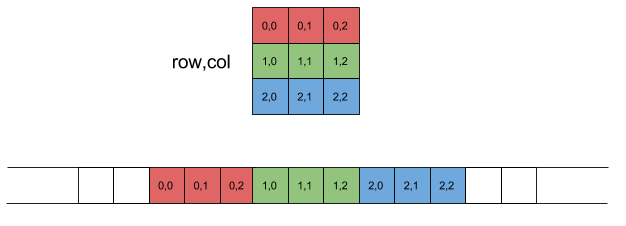
- column-major::
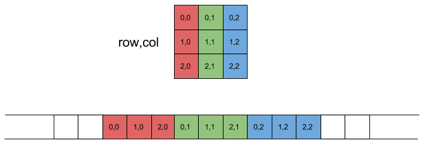
For instance, the following code shows the row-major ordering in c/c++, using old/primitive arrays:
// REF: https://scicomp.stackexchange.com/questions/37264/how-much-space-store-a-matrix-of-numbers
#include <iostream>

int main(int argc, char **argv) {
  const int N = 4;
  int m[N][N] = {0}; //4 by4 matrix with all zeros (default value for ints) allocated on the stack
  for (unsigned int i = 0; i < N; ++i) {
    for (unsigned int j = 0; j < N; ++j) {
      std::cout << &m[i][j] << "\t";
    }
    std::cout << "\n";
  }
  return 0;
}
| 0x16f27ec18 | 0x16f27ec1c | 0x16f27ec20 | 0x16f27ec24 |
| 0x16f27ec28 | 0x16f27ec2c | 0x16f27ec30 | 0x16f27ec34 |
| 0x16f27ec38 | 0x16f27ec3c | 0x16f27ec40 | 0x16f27ec44 |
| 0x16f27ec48 | 0x16f27ec4c | 0x16f27ec50 | 0x16f27ec54 |
Run this on your system. Do you get the same addresses? are they continuous?
In C++, matrices there could be defined in several ways :
Primitive array in the stack (contiguous but limited in size)
double A[M][N];
...
A[2][0] = 59.323;
Primitive dynamic array (not guaranteed to be contiguous in memory):
double **A;
A = new double *[M];
for (int ii = 0; ii < M; ++ii) {
  A[ii] = new double [N];
}
//...
for (int ii = 0; ii < M; ++ii) {
  delete A[ii];
}
delete [] A;
A = nullptr;
A array of arrays : In the stack, limited size
std::array<std::array<double, N>, M> A;
A vector of vectors : not guaranteed to be contiguous in memory
std::vector<std::vector<double>> A;
A.resize(M);
for (int ii = 0; ii < M; ++ii) {
  A[ii].resize(N);
}
All the previous are fine if you don’t care about memory size or contiguous
memory. But in scientific computing, applied to physics, we need to create
performant data structures. For that reason we need to just ask for block of memory
of size M*N and then view it as a 2D array using index tricks.
13.2. 1D and 2D view
Being efficient when accessing memory is key to get a good performance. How are 2D arrays stored in memory? Assume that you have the following 2D array (data inside each cell correspond to indexes)

Given that the ram is 1D, how is that array stored in memory? In c/c++, data is stored in row major (typo in the figure).

Therefore, there must be a given mapping to/from 1D from/to 2D.

For HPC, it is customary to use just 1D arrays to model any 2D (or higher
dimensional) arrays. Instead of using 2D indexes like (i,j) you just use i*N + j,
where N is the number of COLUMNS. For a matrix MxN, what would the (i, j)
index?
This is a bi-dimensional version for filling a given matrix and transposing it.
#include <iostream>
#include <vector>
#include <cstdlib>

void fill_matrix(std::vector<double> & data, int m, int n);
void print_matrix(const std::vector<double> & data, int m, int n);
void transpose_matrix(const std::vector<double> & indata, int m, int n,
                      std::vector<double> & outdata);

int main(int argc, char **argv)
{
  const int M = std::atoi(argv[1]);
  const int N = std::atoi(argv[2]);

  std::vector<double> array2d(M*N, 0.0);

  fill_matrix(array2d, M, N);
  print_matrix(array2d, M, N);

  std::vector<double> array2d_T(M*N, 0.0);
  transpose_matrix(array2d, M, N, array2d_T);
  print_matrix(array2d_T, N, M);

  return 0;
}

void fill_matrix(std::vector<double> & data, int m, int n)
{
  for (int ii = 0; ii < m; ++ii) {
    for (int jj = 0; jj < n; ++jj) {
      data[ii*n + jj] = ii*n+jj; // A_(i, j) = i*n + j = id
    }
  }
}

void print_matrix(const std::vector<double> & data, int m, int n)
{
  for (int ii = 0; ii < m; ++ii) {
    for (int jj = 0; jj < n; ++jj) {
      std::cout << data[ii*n + jj] << " ";
    }
    std::cout << "\n";
  }
  std::cout << "\n";
}

void transpose_matrix(const std::vector<double> & datain, int m, int n,
                      std::vector<double> & dataout)
{
  for (int ii = 0; ii < m; ++ii) {
    for (int jj = 0; jj < n; ++jj) {
      dataout[ii*m + jj] = datain[ii*n + jj]; // Error here
    }
  }
}
| 0 | 1 | 2 | 3 | 4 |
| 5 | 6 | 7 | 8 | 9 |
| 10 | 11 | 12 | 13 | 14 |
| 15 | 16 | 17 | 18 | 19 |
| 0 | 5 | 10 | 15 | |
| 1 | 6 | 11 | 16 | |
| 2 | 7 | 12 | 17 | |
| 3 | 8 | 13 | 18 | |
| 4 | 9 | 14 | 19 | |
13.3. Exercises
For the following exercises, and unless stated otherwise, the size of the matrices must be read from the command line and also the matrices must be filled randomly using a uniform random distribution in [-1, 1]. Also, the random seed must be read from the command line. Furthermore, the solutions must be modularized as follows:
matrix.h- All the functions declarations and includes must come here. Each exercise implies one or more new declarations in this file.
matrix.cpp- All the functions implementations come here.
main_XXXX.cpp- Each exercise will be solved in a main file where the
necessary functions are called. The filename will change (the
XXXXpart).
Then you will need to compile as
g++ -std=c++17 -fsanitize=undefined,address matrix.cpp matrix_XXXX.cpp
Here is a basic example is show for the three files. Remember: the files
matrix.cpp/h will grow with new functions implemented there. The file
main_XXXX.cpp will have a different name for each exercise and call different
functions.
matrix.hDeclarations.
#pragma once
#include <iostream>
#include <vector>
#include <cassert>
#include <random>
void print_matrix(const std::vector<double> & M, int nrows, int ncols);
void fill_matrix_random(std::vector<double> & M, const int nrows, const int ncols, const int seed);
matrix.cppImplementations
#include "matrix.h"
void print_matrix(const std::vector<double> & M, int nrows, int ncols){
    std::cout.setf(std::ios::scientific);
    std::cout.precision(15);

    for (int ii = 0; ii < nrows; ++ii) {
        for (int jj = 0; jj < ncols; ++jj) {
            std::cout << M[ii*ncols + jj] << " "; // (ii, jj) = ii*NCOLS + jj
        }
        std::cout << "\n";
    }
    std::cout << "\n";
}
void fill_matrix_random(std::vector<double> & M, const int nrows, const int ncols, const int seed){
    std::mt19937 gen(seed);
    std::uniform_real_distribution<> dis(-1, 1);
    for (int ii = 0; ii < nrows; ii++){
        for (int jj = 0; jj < ncols; jj++){
            M[ii*ncols + jj] = dis(gen);
        }
    }

}
main_example.cppSimple example
#include "matrix.h"

int main(int argc, char **argv) {
    // read size of matrix
    if (argc != 3) {
        std::cerr << "Error. Usage:\n"
                  << argv[0] << " M N \n"
                  << "M : Rows\n"
                  << "N : Columns\n";
        return 1;
    }
    const int M = std::stoi(argv[1]);
    const int N = std::stoi(argv[2]);

    // create matrix A
    std::vector<double> A(M*N);

    // fill matrix randomly
    fill_matrix_random(A, M, N, 0); // 0 == seed

    // print matrix
    print_matrix(A, M, N);

    return 0;
}
Please solve the following:
- Trace of a matrix: Compute the trace of a random matrix using 1D indexing.
- Hilbert matrix: Create a function to compute the trace of that matrix. Fill the matrix as the Hilbert Matrix, \(A_{ij} = 1/(i +j +1)\)
- Implement matrix-matrix multiplication. A function must received the two input matrices and an output matrix and write there the result.
- Implement a function to compute the matrix multiplication of matrix with its transpose.
- Implement a function to compute the power of a matrix performing successive multiplications.
- Implement a function that receives a matrix and a power and checks if it is idempotent under some precision, that is, if \(|A^p - A| < \epsilon\), where the norm is evaluated checking the inequality element-by-element.
- Implement a function that receives two matrices and check if they are inverse of each other, that is , if \(|AB - I| < \epsilon\) and \(|BA - I| < \epsilon\), where the check is done on each element.
- Write a function that receives two matrices and checks if they commute under a given precision, that is , \(|AB - BA| < \epsilon\).
- Implement a function that receives a matrix and checks if it is orthogonal, that is, if \(|A A^T - I| < \epsilon\), where the norm is evaluated checking the inequality element-by-element.
- Implement a function that receives a matrix OF COMPLEX NUMBERS and checks if it is hermitian,
that is, if \(|A A^\dagger - I| < \epsilon\), where the norm is evaluated checking the
inequality element-by-element. Use the
<complex>header. \(A^\dagger\) means the transpose conjugate. - Write a function that receives three components of a vectors and saves the corresponding Pauli-vector-matrix: https://en.wikipedia.org/wiki/Pauli_matrices#Pauli_vector
- Extend your multiplication routine to use complex numbers and check the Pauli matrix commutation relations: https://en.wikipedia.org/wiki/Pauli_matrices#(Anti-)Commutation_relations
- Write a routine to fill a matrix as a Vandermonde matrix, https://en.wikipedia.org/wiki/Vandermonde_matrix , and then compute and print its trace Read the number of rows from the command line
- Implement a function that receives a matrix and an array representing the coefficients of a polynomial, \(a_0, a_1, \ldots, a_n\), and evaluates that polynomial on the given matrix, \(a_0 I + a_1 A + a_2 A^2 + \ldots + a_n A^n\), and stores the result in an output matrix.
Matrix multiplication time: Explore how the total multiplication time grows with the matrix size. The following code is a template. You should read it and understand it carefully. Implement what is needed.
    #include <iostream>
    #include <chrono>
    #include <random>
    #include <cmath>
    #include <cstdlib>
    #include <vector>
    #include <algorithm>

    void multiply(const std::vector<double> & m1, const std::vector<double> & m2, std::vector<double> & m3);

    int main(int argc, char **argv) {
      // read parameters
      const int N = std::atoi(argv[1]);
      const int SEED = std::atoi(argv[2]);

      // data structs
      std::vector<double> A(N*N, 0.0), B(N*N, 0.0), C(N*N, 0.0);

      // fill matrices A and B, using random numbers betwwen 0 and 1
      std::mt19937 gen(SEED);
      std::uniform_real_distribution<> dist(0.,1.);
      // lambda function: a local function that captures [] something, receives something (), and return something {}
      // See: https://www.learncpp.com/cpp-tutorial/introduction-to-lambdas-anonymous-functions/
      std::generate(A.begin(), A.end(), [&gen, &dist](){ return dist(gen); }); // uses a lambda function
      std::generate(B.begin(), B.end(), [&gen, &dist](){ return dist(gen); }); // uses a lambda function

      // multiply the matrices A and B and save the result into C. Measure time
      auto start = std::chrono::high_resolution_clock::now();
      multiply(A, B, C);
      auto stop = std::chrono::high_resolution_clock::now();

      // use the matrix to avoid the compiler removing it
      std::cout << C[N/2] << std::endl;

      // print time
      auto elapsed = std::chrono::duration<double>(stop - start);
      std::cout << elapsed.count() << "\n";

      return 0;
    }

    // implementations
    void multiply(const std::vector<double> & m1, const std::vector<double> & m2, std::vector<double> & m3)
    {
      const int N = std::sqrt(m1.size()); // assumes square matrices
      delete this line and implement the matrix multiplication here
    }
When run as
./a.out 64 10
you should get something like
14.6676 0.002486 or when run as
./a.out 256 10
you should get something like
Plot, in log-log scale, the time as a function of the matriz size \(N\) in the range \(N \in \{4, 8, 16, 32, 64, 128, 256, 512, 1024\}\). Normalize all times by the time at \(N = 4\).
14. Vector operations: Coefficient-wise
Coefficient-wise operations, like the vector sum (which operate component by
component), are very common and useful. For instance, the whole numpy library
is based on that (https://numpy.org/doc/stable/user/basics.broadcasting.html).
In c++ you can also do it, and it simplifies a lot many operations related to
vectors. You have two options: using the standard library valarray, or using
Eigen array.
14.1. C++ valarray
You can find the reference implementation at https://en.cppreference.com/w/cpp/numeric/valarray .
#include <iostream>
#include <valarray>
#include <cmath>

int main()
{
    std::valarray<int> v = {1,2,3,4,5,6,7,8,9,10};

    double suma = v.sum();

    std::cout << suma << "\n";

    return 0;
}
Exercise: Como usar la utilidad apply para multiplicar todos los elementos por 2 si el numero es impar y por 3 si el numero es par A simple example for indexing, is the following (https://en.cppreference.com/w/cpp/numeric/valarray/operator%3D)
#include <iomanip>
#include <iostream>
#include <valarray>

void print(const char* rem, const std::valarray<int>& v)
{
    std::cout << std::left << std::setw(36) << rem << std::right;
    for (int n: v) std::cout << std::setw(3) << n;
    std::cout << '\n';
}

int main()
{
    std::valarray<int> v1(3);
    v1 = -1; // (3) from a scalar
    print("assigned from scalar: ", v1);

    v1 = {1, 2, 3, 4, 5, 6}; // (8): from initializer list of different size
    print("assigned from initializer_list:", v1);

    std::valarray<int> v2(3);
    v2 = v1[std::slice(0,3,2)]; // (4): from slice array
    print("every 2nd element starting at pos 0:", v2);

    v2 = v1[v1 % 2 == 0]; // (6): from mask array
    print("values that are even:", v2);

    std::valarray<std::size_t> idx = {0,1,2,4}; // index array
    v2.resize(4); // sizes must match when assigning from gen subscript
    v2 = v1[idx]; // (7): from indirect array
    print("values at positions 0, 1, 2, 4:", v2);

    return 0;
}
| assigned | from | scalar: | -1 | -1 | -1 | |||||
| assigned | from | initializerlist: | 1 | 2 | 3 | 4 | 5 | 6 | ||
| every | 2nd | element | starting | at | pos | 0: | 1 | 3 | 5 | |
| values | that | are | even: | 2 | 4 | 6 | ||||
| values | at | positions | 0, | 1, | 2, | 4: | 1 | 2 | 3 | 5 |
As you can see, all operations are done at the element level. You can also define masks:
#include <iostream>
#include <valarray>

int main()
{
  std::valarray<int> data = {0,1,2,3,4,5,6,7,8,9};

  std::cout << "Initial valarray: ";
  for(int n: data) std::cout << n << ' ';
  std::cout << '\n';

  data[data > 5] = -1; // valarray<bool> overload of operator[]
  // the type of data>5 is std::valarray<bool>
  // the type of data[data>5] is std::mask_array<int>

  std::cout << "After v[v>5]=-1:  ";
  for(std::size_t n = 0; n < data.size(); ++n)
    std::cout << data[n] << ' ';  // regular operator[]
  std::cout << '\n';
}
| Initial | valarray: | 0 | 1 | 2 | 3 | 4 | 5 | 6 | 7 | 8 | 9 |
| After | v[v>5]=-1: | 0 | 1 | 2 | 3 | 4 | 5 | -1 | -1 | -1 | -1 |
There is also a nice utility, apply, that you can use to apply a function to
each element:
#include <iostream>
#include <valarray>
#include <cmath>

int main()
{
    std::valarray<int> v = {1,2,3,4,5,6,7,8,9,10};
    v = v.apply([](int n)->int {
                    return std::round(std::tgamma(n+1));
                });
    for(auto n : v) {
        std::cout << n << ' ';
    }
    std::cout << '\n';
}
1 2 6 24 120 720 5040 40320 362880 3628800
14.1.1. Exercises
- Create a program that computes the dot product among two vectors using valarray. Your program must read the vector size from the command line. Fill them using any function you want.
- Is a valarray in the heap or the stack? Verify (check https://en.cppreference.com/w/cpp/numeric/valarray/resize)
- Using the overloaded operators create a valarray for N=1000 points between 0 and \(2\pi\), then compute the \(\sin\) of those numbers and assing the result to a another valarray, and finally print only the values that fulfill that \(|\sin x| \le 0.5\). All of this without using loops.
If you discretize time in steps of size \(\delta t\), and you have the forces on a given ideal particle, you can compute the next position using the Euler algorithm,
\begin{align} \vec R(t+\delta t) &= \vec R(t) + \delta t \vec V(t),\\ \vec V(t + \delta t) &= \vec V(t) + \delta t \vec F(t)/m.\\ \end{align}Use valarrays to model the vectors. Compute the trayectory of a particle of mass \(m=0.987\), with initial conditions \(\vec R(0) = (0, 0, 4.3), V(0) = (0.123, 0.0, 0.98)\), under the influence of gravity. Plot it. Later add some damping. Later add some interaction with the ground.
14.2. Eigen arrays
This library also implements element-wise operations and data structs, https://eigen.tuxfamily.org/dox/group__TutorialArrayClass.html , https://eigen.tuxfamily.org/dox/group__QuickRefPage.html#title6 . There are many overloaded operations that you can use. Plase check the docs.
This is an example of a sum, element-wise
#include <eigen3/Eigen/Dense>
#include <iostream>

int main()
{
  Eigen::ArrayXXf a(3,3);
  Eigen::ArrayXXf b(3,3);
  a << 1,2,3,
       4,5,6,
       7,8,9;
  b << 1,2,3,
       1,2,3,
       1,2,3;

  // Adding two arrays
  std::cout << "a + b = " << std::endl << a + b << std::endl << std::endl;

  // Subtracting a scalar from an array
  std::cout << "a - 2 = " << std::endl << a - 2 << std::endl;
}
| a | + | b | = |
| 2 | 4 | 6 | |
| 5 | 7 | 9 | |
| 8 | 10 | 12 | |
| a | - | 2 | = |
| -1 | 0 | 1 | |
| 2 | 3 | 4 | |
| 5 | 6 | 7 |
and this an example for vector product
#include <eigen3/Eigen/Dense>
#include <iostream>

int main()
{
  Eigen::ArrayXXf a(2,2);
  Eigen::ArrayXXf b(2,2);
  a << 1,2,
       3,4;
  b << 5,6,
       7,8;
  std::cout << "a * b = " << std::endl << a * b << std::endl;
}
| a | * | b | = |
| 5 | 12 | ||
| 21 | 32 |
More operations:
#include <eigen3/Eigen/Dense>
#include <iostream>

int main()
{
  Eigen::ArrayXf a = Eigen::ArrayXf::Random(5);
  a *= 2;
  std::cout << "a =" << std::endl
            << a << std::endl;
  std::cout << "a.abs() =" << std::endl
            << a.abs() << std::endl;
  std::cout << "a.abs().sqrt() =" << std::endl
            << a.abs().sqrt() << std::endl;
  std::cout << "a.min(a.abs().sqrt()) =" << std::endl
            << a.min(a.abs().sqrt()) << std::endl;
}
| a | = |
| -1.99997 | |
| -1.47385 | |
| 1.02242 | |
| -0.165399 | |
| 0.131069 | |
| a.abs() | = |
| 1.99997 | |
| 1.47385 | |
| 1.02242 | |
| 0.165399 | |
| 0.131069 | |
| a.abs().sqrt() | = |
| 1.4142 | |
| 1.21402 | |
| 1.01115 | |
| 0.406693 | |
| 0.362034 | |
| a.min(a.abs().sqrt()) | = |
| -1.99997 | |
| -1.47385 | |
| 1.01115 | |
| -0.165399 | |
| 0.131069 |
14.2.1. Exercises:
Solve the same previous exercises used on valarray
15. Numerical Libraries
15.1. Eigen Library: Introduction
http://eigen.tuxfamily.org/index.php?title=Main_Page
Start by: http://eigen.tuxfamily.org/dox/GettingStarted.html
First example from the tutorial:
// First example on how to use eigen
// compile with: g++ -std=c++11 -I /usr/include/eigen3 17-eigen-example01.cpp
#include <iostream>
#include <eigen3/Eigen/Dense>

int main(int argc, char **argv)
{
  // X = Dynamic size
  // d = double
  Eigen::MatrixXd m(2,2);
  m(0,0) = 3;
  m(1,0) = 2.5;
  m(0,1) = -1;
  m(1,1) = m(1,0) + m(0,1);
  std::cout << m << std::endl;

  return 0;
}
Second example from the tutorial: Matrix-vector multiplication
// Second example, slighlty modified to include namespaces explicitly
#include <iostream>
#include <eigen3/Eigen/Dense>

using EMXd = Eigen::MatrixXd;

int main(int argc, char **argv)
{
  Eigen::MatrixXd m = Eigen::MatrixXd::Random(3,3); // EMXd m = EMXd::Random(3,3);
  m = (m + Eigen::MatrixXd::Constant(3,3,1.2)) * 50;
  std::cout << "m =" << std::endl << m << std::endl;
  Eigen::VectorXd v(3);
  v << 1, 2, 3;
  std::cout << "m * v =" << std::endl << m * v << std::endl;

  return 0;
}
15.1.1. Exercises
- Read the matrix rows and columns from the command line.
- Find in the documentation how to compute the inverse. Write a program that
creates a random matrix, compute its inverse, then multiplies then and
finally prints the firts element of the resulting matrix. For a matriz of
size 1000, is there any difference when you compile normally and when you use
-O3?
15.2. Eigen: Linear Algebra
15.2.1. Householder QR for \(Ax=b\)
In this example we are going to use eigen to solve the system \(\boldsymbol{A}\vec x = \vec{x}\) using HouseHolder QR decomposition as done in http://eigen.tuxfamily.org/dox/group__TutorialLinearAlgebra.html .
#include <iostream>
#include <eigen/Eigen/Dense>

int main()
{
  Eigen::Matrix3f A;
  Eigen::Vector3f b;
  A << 1,2,3,  4,5,6,  7,8,10;
  b << 3, 3, 4;
  std::cout << "Here is the matrix A:\n" << A << std::endl;
  std::cout << "Here is the vector b:\n" << b << std::endl;
  Eigen::Vector3f x = A.colPivHouseholderQr().solve(b);
  std::cout << "The solution is:\n" << x << std::endl;
  std::cout << "Verification:\n" << (A*x - b).norm() << std::endl;
}
With double :
#include <iostream>
#include <eigen/Eigen/Dense>

int main()
{
  Eigen::Matrix3d A;
  Eigen::Vector3d b;
  A << 1,2,3,  4,5,6,  7,8,10;
  b << 3, 3, 4;
  std::cout << "Here is the matrix A:\n" << A << std::endl;
  std::cout << "Here is the vector b:\n" << b << std::endl;
  Eigen::Vector3d x = A.colPivHouseholderQr().solve(b);
  std::cout << "The solution is:\n" << x << std::endl;
  std::cout << "Verification:\n" << (A*x - b).norm() << std::endl;
}
Exercise: Compute the same solution for a 1000x1000 matrix (read the size from the command line). Use a random amtrix and vector.
15.2.2. LU decomposition for \(Ax = b\)
The following code shows how to perform a LU decomposition and use it to solve it a linear problem:
#include <iostream>
#include <Eigen/Dense>

void solvesystem(int size);

int main(int argc, char ** argv)
{
  const int M = atoi(argv[1]); // Matrix size
  solvesystem(M);
}

void solvesystem(int size)
{
  Eigen::MatrixXd A = Eigen::MatrixXd::Random(size, size);
  Eigen::MatrixXd b = Eigen::MatrixXd::Random(size, 1);
  Eigen::MatrixXd x = A.fullPivLu().solve(b); // magic
  double relative_error = (A*x - b).norm() / b.norm(); // norm() is L2 norm
  std::cout << A << std::endl;
  std::cout << b << std::endl;
  std::cout << "The relative error is:\n" << relative_error << std::endl;
}
| -0.999984 | -0.562082 | -0.232996 | 0.0594004 | -0.165028 |
| -0.736924 | -0.905911 | 0.0388327 | 0.342299 | 0.373545 |
| 0.511211 | 0.357729 | 0.661931 | -0.984604 | 0.177953 |
| -0.0826997 | 0.358593 | -0.930856 | -0.233169 | 0.860873 |
| 0.0655345 | 0.869386 | -0.893077 | -0.866316 | 0.692334 |
| 0.0538576 | ||||
| -0.81607 | ||||
| 0.307838 | ||||
| -0.168001 | ||||
| 0.402381 | ||||
| The | relative | error | is: | |
| 1.18763e-15 |
15.2.3. Eigenvalue problems
Following the documentation of the general eigen solveer, https://eigen.tuxfamily.org/dox/classEigen_1_1EigenSolver.html, we can use the example to show how it works:
#include <iostream>
#include <cstdlib>
#include <Eigen/Dense>
#include <complex>

int main(int argc, char **argv) {
  const int N = std::atoi(argv[1]);

  Eigen::MatrixXd A = Eigen::MatrixXd::Random(N,N);
  std::cout << "Here is a random matrix, A:" << std::endl << A << std::endl << std::endl;

  Eigen::EigenSolver<Eigen::MatrixXd> es(A);
  std::cout << "The eigenvalues of A are:" << std::endl << es.eigenvalues() << std::endl;
  std::cout << "The matrix of eigenvectors, V, is:" << std::endl << es.eigenvectors() << std::endl << std::endl;

  std::complex<double> lambda = es.eigenvalues()[0];
  std::cout << "Consider the first eigenvalue, lambda = " << lambda << std::endl;
  Eigen::VectorXcd v = es.eigenvectors().col(0);
  std::cout << "If v is the corresponding eigenvector, then lambda * v = " << std::endl << lambda * v << std::endl;
  std::cout << "... and A * v = " << std::endl << A.cast<std::complex<double> >() * v << std::endl << std::endl;

  Eigen::MatrixXcd D = es.eigenvalues().asDiagonal();
  Eigen::MatrixXcd V = es.eigenvectors();
  std::cout << "Finally, V * D * V^(-1) = " << std::endl << V * D * V.inverse() << std::endl;

  return 0;
}
| Here | is | a | random | matrix, | A: | |||||
| -0.999984 | -0.905911 | 0.661931 | -0.233169 | 0.692334 | 0.820642 | |||||
| -0.736924 | 0.357729 | -0.930856 | -0.866316 | 0.0538576 | 0.524396 | |||||
| 0.511211 | 0.358593 | -0.893077 | -0.165028 | -0.81607 | -0.475094 | |||||
| -0.0826997 | 0.869386 | 0.0594004 | 0.373545 | 0.307838 | -0.905071 | |||||
| 0.0655345 | -0.232996 | 0.342299 | 0.177953 | -0.168001 | 0.472164 | |||||
| -0.562082 | 0.0388327 | -0.984604 | 0.860873 | 0.402381 | -0.343532 | |||||
| The | eigenvalues | of | A | are: | ||||||
| (-1.49257,0) | ||||||||||
| (0.0766151,1.15956) | ||||||||||
| (0.0766151,-1.15956) | ||||||||||
| (0.733141,0) | ||||||||||
| (-0.53356,0.220193) | ||||||||||
| (-0.53356,-0.220193) | ||||||||||
| The | matrix | of | eigenvectors, | V, | is: | |||||
| (0.786312,0) | (-0.263017,0.312691) | (-0.263017,-0.312691) | (0.152242,0) | (0.325234,-0.366548) | (0.325234,0.366548) | |||||
| (0.0306896,0) | (0.35708,0.148567) | (0.35708,-0.148567) | (-0.696683,0) | (0.0186831,0.157674) | (0.0186831,-0.157674) | |||||
| (-0.576577,0) | (0.246839,-0.0954089) | (0.246839,0.0954089) | (0.157239,0) | (-0.0561259,0.314894) | (-0.0561259,-0.314894) | |||||
| (-0.0522699,0) | (-0.00740087,-0.598314) | (-0.00740087,0.598314) | (-0.351252,0) | (-0.0994047,0.310235) | (-0.0994047,-0.310235) | |||||
| (0.169033,0) | (-0.175843,0.159214) | (-0.175843,-0.159214) | (-0.119052,0) | (0.304502,-0.552123) | (0.304502,0.552123) | |||||
| (-0.13049,0) | (-0.445552,-0.0247806) | (-0.445552,0.0247806) | (-0.573742,0) | (0.0639622,0.352941) | (0.0639622,-0.352941) | |||||
| Consider | the | first | eigenvalue, | lambda | = | (-1.49257,0) | ||||
| If | v | is | the | corresponding | eigenvector, | then | lambda | * | v | = |
| (-1.17363,0) | ||||||||||
| (-0.0458064,0) | ||||||||||
| (0.860581,-0) | ||||||||||
| (0.0780164,-0) | ||||||||||
| (-0.252293,0) | ||||||||||
| (0.194765,-0) | ||||||||||
| … | and | A | * | v | = | |||||
| (-1.17363,0) | ||||||||||
| (-0.0458064,0) | ||||||||||
| (0.860581,0) | ||||||||||
| (0.0780164,0) | ||||||||||
| (-0.252293,0) | ||||||||||
| (0.194765,0) | ||||||||||
| Finally, | V | * | D | * | V(-1) | = | ||||
| (-0.999984,2.22045e-16) | (-0.905911,0) | (0.661931,-1.11022e-16) | (-0.233169,3.05311e-16) | (0.692334,1.38778e-16) | (0.820642,-6.93889e-17) | |||||
| (-0.736924,1.38778e-17) | (0.357729,-7.63278e-17) | (-0.930856,-2.22045e-16) | (-0.866316,9.02056e-17) | (0.0538576,5.55112e-17) | (0.524396,-8.67362e-19) | |||||
| (0.511211,-1.94289e-16) | (0.358593,-3.1225e-17) | (-0.893077,-5.55112e-17) | (-0.165028,-1.66533e-16) | (-0.81607,-1.38778e-16) | (-0.475094,6.93889e-17) | |||||
| (-0.0826997,-2.77556e-17) | (0.869386,7.63278e-17) | (0.0594004,5.55112e-17) | (0.373545,-1.94289e-16) | (0.307838,-1.11022e-16) | (-0.905071,1.07553e-16) | |||||
| (0.0655345,-1.11022e-16) | (-0.232996,0) | (0.342299,1.11022e-16) | (0.177953,1.11022e-16) | (-0.168001,8.32667e-17) | (0.472164,-5.55112e-17) | |||||
| (-0.562082,-1.11022e-16) | (0.0388327,2.42861e-17) | (-0.984604,0) | (0.860873,-5.55112e-17) | (0.402381,-1.11022e-16) | (-0.343532,3.46945e-17) |
15.2.4. Profiling
Now, we will measure the time spent computing the solution. To do so we will use the chrono library
#include <iostream>
#include <chrono>
#include <Eigen/Dense>


void solvesystem(int size);

int main(int argc, char ** argv)
{
  const int M = atoi(argv[1]); // Matrix size
  const int S = atoi(argv[2]); // seed
  srand(S); // control the seed

  solvesystem(M);
}

void solvesystem(int size)
{
  Eigen::MatrixXd A = Eigen::MatrixXd::Random(size, size);
  Eigen::MatrixXd b = Eigen::MatrixXd::Random(size, 1);

  auto start = std::chrono::steady_clock::now();
  Eigen::MatrixXd x = A.fullPivLu().solve(b);
  auto end   = std::chrono::steady_clock::now();

  std::chrono::duration<double> elapsed_seconds = end-start;
  std::cout << size*size << "\t" << elapsed_seconds.count() << "\t" << x(0) << std::endl;
}
| 10000 | 0.026181 | -2.18851 |
If you repeat several times, you will get different times. It would be better to compute simple statistics on this:
#include <iostream>
#include <chrono>
#include <cmath>
#include <Eigen/Dense>

double solvesystem(int size);

int main(int argc, char ** argv)
{
  const int N = atoi(argv[1]); // Matrix size
  const int S = atoi(argv[2]); // Seed
  const int R = atoi(argv[3]); // Reps

  double sum = 0, sum2 = 0;
  double time = 0;
  for (int rep = 0; rep < R; ++rep) {
    srand(S+rep);
    time = solvesystem(N);
    sum  += time;
    sum2 += time*time;
  }
  double mean = sum/R;
  double sigma = std::sqrt(R*(sum2/R - mean*mean)/(R-1));

  std::cout.setf(std::ios::scientific); std::cout.precision(15);
  std::cout << N*N << "\t" << mean << "\t" << sigma << std::endl;

  return 0;
}

double solvesystem(int size)
{
  Eigen::MatrixXd A = Eigen::MatrixXd::Random(size, size);
  Eigen::MatrixXd b = Eigen::MatrixXd::Random(size, 1);

  auto start = std::chrono::steady_clock::now();
  Eigen::MatrixXd x = A.fullPivLu().solve(b);
  auto end   = std::chrono::steady_clock::now();

  std::chrono::duration<double> elapsed_seconds = end-start;
  return elapsed_seconds.count();
}
| 10000 | 0.0167343584 | 0.002405873881085173 |
15.3. GSL : Gnu Scientific Library
https://www.gnu.org/software/gsl/ Documentation: https://www.gnu.org/software/gsl/doc/html/index.html
15.3.1. Special functions example : Bessel function
See: https://www.gnu.org/software/gsl/doc/html/specfunc.html
// Adapted to c++ from : https://www.gnu.org/software/gsl/doc/html/specfunc.html
                                 // compile as: g++ 17-gsl-bessel.cpp -lgsl -lgslcblas
#include <cstdio>
#include <gsl/gsl_sf_bessel.h>

int main (void)
{
  double x = 5.0;
  double expected = -0.17759677131433830434739701;

  double y = gsl_sf_bessel_J0 (x);

  printf ("J0(5.0) = %.18f\n", y);
  printf ("exact   = %.18f\n", expected);
  return 0;
}
Exercise: Write a program that prints the Bessel function of order zero for \(x \in [0, 10]\) in steps \(\Delta x = 0.01\). Plot it.
// Adapted to c++ from : https://www.gnu.org/software/gsl/doc/html/specfunc.html
                                 // compile as: g++ 17-gsl-bessel-exercise.cpp -lgsl -lgslcblas
#include <iostream>
#include <gsl/gsl_sf_bessel.h>

int main (void)
{
  const double DX = 0.01;
  for(int ii = 0; ii <= 4000; ++ii) {
    double x = 0 + ii*DX;
    std::cout << x << "    " << gsl_sf_bessel_J0(x) << "\n";
  }

  return 0;
}
15.4. Exercises
- Check presentation.
When solving the laplace equation \(\nabla V = 0\) to compute the electrostatic potential on a planar region, you can discretize the derivatives on a grid and then arrive to the following equation
\begin{equation} V_{i+1,j} + V_{i-1,j} + V_{i,j+1} + V_{i,j-1} - 4V_{i,j} = 0.0. \end{equation}This can be written as a matrix problem. Solve the matrix problem for a square plate of lenght \(L\), with \(N\) points on each side. The boundary conditions, of Dirichlet type, are \(V(x, 0) = 5\sin(\pi x/L)\), \(V(x, L) = V(0, y) = V(L, y) = 0.0\).
- Compute the determinant of the Vandermonde matrix of size \(N\times N\). Measure the time as a function of \(N\).
- Compute the condition number for an arbitrary matrix \(A\). Apply it for the Vandermonde matrix. The condition number is defined as \(\kappa(A) = |A^{-1}| |A|\)
- Compute the eigen values and the condition number for the Hilber matrix.
- Define a rotation matrix in 2d by an angle \(\theta\). Apply it to a given vector and check that it is actually rotated.
- Check how to implement complex matrices in Eigen.
- Apply the power method to compute the maximum eigen value of the Vandermonde matrix (or any other matrix).
- Imagine that you have two masses \(m_1, m_2\), coupled through springs in the form wall-spring-mass-spring-mass-spring-wall. All spring are linear with constant \(k\). Write the equations of motion, replace each solution with \(x_i(t) = A_i e^{i\omega t}\), and obtain a matrix representation to get the amplitudes. Compute the eigen values and eigen-vectors. Those are the normal modes . Extend to n oscillators of the same mass.
16. Primitive arrays, pointers and manual memory managment
16.1. Motivation
They are used extensively in HPC:
- Cuda programming:
- Super computing - Distributed memory:
16.2. Primitive arrays
16.2.1. Definition
- Variables del mismo tipo y contiguas en memoria
- Índices comienzan en cero, y van hasta N-1
- Siempre compilar con sanitizers:
-fsanitize=address -fsanitize=undefined -fsanitize=leak
// g++ -g -fsanitize=address
#include <iostream>

int main(void)
{
    const int N = 10;
    double data[N] = {1, 2, 3}; // Se inicializan unos, los demas en cero
    std::cout << data[0] << std::endl;
    std::cout << data[N-1] << std::endl;
    std::cout << data << std::endl;
    std::cout << &data[0] << std::endl;
    // std::cout << data[N] << std::endl; // BAD
    // std::cout << data[-1] << std::endl; // BAD

}
| 1 |
| 0 |
| 0x16f7bebf8 |
| 0x16f7bebf8 |
// g++ -g -fsanitize=address
#include <iostream>

int main(void)
{
    const int N = 10;

    double data[N]= {0};
    //std::cout << data[0] << std::endl;
    //std::cout << data[N-1] << std::endl;
    //std::cout << data[N] << std::endl; // wrong

// initialize the array with even numbers
    for(int ii = 0; ii < N; ++ii){
        data[ii] = 2*ii;
    }

// print the array
    for(int ii = 0; ii < N; ++ii){
        std::cout << data[ii] << std::endl;
    }

// compute mean
    double sum = 0.0;
    for(int ii = 0; ii < N; ++ii){
        sum += data[ii];
    }
    std::cout << "Average = " << sum/N << std::endl;
}
| 0 | ||
| 2 | ||
| 4 | ||
| 6 | ||
| 8 | ||
| 10 | ||
| 12 | ||
| 14 | ||
| 16 | ||
| 18 | ||
| Average | = | 9 |
16.2.2. Calling a function with arrays
Goal: create functions and pass arrays by reference.
[X]Let’s create a function that receives our vectors and returns their dot product.[X]Also create a function to initialize the vectors[X]Create a function print them.
Passing primitive arrays to functions require to declare the arguments as
double a[] (for 1d arrays)
// Computing dot product
#include <iostream>

double dotproduct(const double a1[], const double a2[], int size); // by reference by default
void init(double a1[], double a2[], int size); // by reference by default
void print(const double array[], int size);

int main(int argc, char **argv)
{
    // double x1 = 9.87, y1 = -0.65, z1 = 7.65432;
    // double x2 = -5.432, y2 = -0.6598876, z2 = -0.64359;
    //std::cout << x1*x2 + y1*y2 + z1*z2 << std::endl;

    // memoria = stack(estatico) + heap(dinamica)

    // primitive arrays //limited by stack size
    int N = 10000;
    double v1[N]{9.87, -0.65, 7.65432}, v2[N]{-5.432, -0.6598876, -0.64359};
    init(v1, v2, N);
    std::cout << dotproduct(v1, v2, N) << std::endl;
    print(v1, 10);
    print(v2, 11);

    return 0;
}

double dotproduct(const double a1[], const double a2[], int size)
{
    double dot = 0;
    for (int ii = 0; ii < size; ii++) {
        dot += a1[ii]*a2[ii];
    }
    return dot;
}
void init(double a1[], double a2[], int size)
{
    for (int ii = 0; ii < size; ii++) {
        a1[ii] = 2*ii;
        a2[ii] = 1.0/(2*ii*ii + 1);
    }
}

void print(const double array[], int size)
{
    for (int ii = 0; ii < size; ii++) {
        std::cout << array[ii] << " " ;
    }
    std::cout << "\n";
}
9.36144
#include <iostream>

//   por defecto, los arreglos primitivos se pasan por referencia
void initialize(double xdata[], int size);
void print(const double xdata[], int size);
void print_average(const double xdata[], int size);

int main(void)
{
  const int N = 10;
  double data[N]{0};

  // initialize the array with even numbers
  initialize(data, N);

  // print the array
  print(data, N);

  // compute mean
  print_average(data, N);

  return 0;
}


void print(const double xdata[], int size)
{
  // print the array
  for(int ii = 0; ii < size; ++ii){
    std::cout << xdata[ii] << std::endl;
  }
}

void print_average(const double xdata[], int size)
{
  double sum = 0.0;
  for(int ii = 0; ii < size; ++ii){
    sum += xdata[ii];
  }
  std::cout << "Average = " << sum/size << std::endl;
}

void initialize(double xdata[], int size)
{
  for(int ii = 0; ii < size; ++ii){
    xdata[ii] = 2*ii;
  }
}
| 0 | ||
| 2 | ||
| 4 | ||
| 6 | ||
| 8 | ||
| 10 | ||
| 12 | ||
| 14 | ||
| 16 | ||
| 18 | ||
| Average | = | 9 |
- DONE Matrix transpose
Write a program that computes the transpose of a matrix
#include <iostream>

int main(void)
{
const int N = 4;

double matrix[N*N] = {0}, matrixT[N*N] = {0};

// fill matrix
for (int ii = 0; ii < N; ++ii) {
   for (int jj = 0; jj < N; ++jj) {
       matrix[ii*N + jj] = ii*N + jj;
   }
}

// transpose and store into matrixT
for (int ii = 0; ii < N; ++ii) {
   for (int jj = 0; jj < N; ++jj) {
       matrixT[ii*N + jj] = matrix[jj*N + ii];
   }
}

// print the matrices
std::cout << "Original matrix:\n";
for (int ii = 0; ii < N; ++ii) {
   for (int jj = 0; jj < N; ++jj) {
       std::cout << matrix[ii*N + jj] <<  "  ";
   }
   std::cout << "\n";
}

std::cout << "Transposed matrix:\n";
for (int ii = 0; ii < N; ++ii) {
   for (int jj = 0; jj < N; ++jj) {
       std::cout << matrixT[ii*N + jj] <<  "  ";
   }
   std::cout << "\n";
}

return 0;
}
Original matrix: 0 1 2 3 4 5 6 7 8 9 10 11 12 13 14 15 Transposed matrix: 0 4 8 12 1 5 9 13 2 6 10 14 3 7 11 15 #include <iostream> #include <vector> int main(void) { const int N = 4; std::vector<double> matrix, matrixT; matrix.resize(N*N); matrixT.resize(N*N); // fill matrix for (int ii = 0; ii < N; ++ii) { for (int jj = 0; jj < N; ++jj) { matrix[ii*N + jj] = ii*N + jj; } } // transpose and store into matrixT for (int ii = 0; ii < N; ++ii) { for (int jj = 0; jj < N; ++jj) { matrixT[ii*N + jj] = matrix[jj*N + ii]; } } // print the matrices std::cout << "Original matrix:\n"; for (int ii = 0; ii < N; ++ii) { for (int jj = 0; jj < N; ++jj) { std::cout << matrix[ii*N + jj] << " "; } std::cout << "\n"; } std::cout << "Transposed matrix:\n"; for (int ii = 0; ii < N; ++ii) { for (int jj = 0; jj < N; ++jj) { std::cout << matrixT[ii*N + jj] << " "; } std::cout << "\n"; } return 0; }
Original matrix: 0 1 2 3 4 5 6 7 8 9 10 11 12 13 14 15 Transposed matrix: 0 4 8 12 1 5 9 13 2 6 10 14 3 7 11 15
16.3. Pointers
16.3.1. Basic pointers
Goal: to learn what a pointer is (a variable that stores a memory address) and its relationship with primitive arrays
Let’s first check a key result comming from the addresses of the name and the first element in a primitive array
#include <iostream>

int main(void)
{
  int a = 67;
  int * ptr = nullptr;

  ptr = &a;

  std::cout << a << std::endl;
  std::cout << &a << std::endl;

  std::cout << ptr << std::endl;
  std::cout << *ptr << std::endl;
  std::cout << &ptr << std::endl;

  *ptr = 32; // igual a hacer a = 32;
  std::cout << a << std::endl;

  return 0;
}
| 67 |
| 0x7ffee30060ec |
| 0x7ffee30060ec |
| 67 |
| 0x7ffee30060e0 |
| 32 |
A more elaborated example shows how to “jump” in memory by incrementing a pointer
#include <iostream>

int main(int argc, char **argv) {
    double val = 0.987766;
    double * ptr = nullptr; // pointer. Only stores memory addresses
    ptr = &val; // ptr stores x memory address
    //ptr = val; // error, cannot store common values
    std::cout << "val  : " << val  << std::endl;
    std::cout << "&val : " << &val << std::endl;
    std::cout << "ptr  : " << ptr  << std::endl; // prints val address
    std::cout << "*ptr : " << *ptr << std::endl; // prints val VALUE
    std::cout << "&ptr : " << &ptr << std::endl; // prints ptr address
    std::cout << "*(ptr+0) : " << *(ptr+0) << std::endl; // value pointed by ptr
    std::cout << "*(ptr+1) : " << *(ptr+1) << std::endl; // value one jump later
    std::cout << "ptr[0] : " << ptr[0] << std::endl; //

    return 0;
}
| val | : | 0.987766 |
| &val | : | 0x7ffeea3c50e8 |
| ptr | : | 0x7ffeea3c50e8 |
| *ptr | : | 0.987766 |
| &ptr | : | 0x7ffeea3c50e0 |
| *(ptr+0) | : | 0.987766 |
| *(ptr+1) | : | 6.95313e-310 |
| ptr[0] | : | 0.987766 |
C++/Python tutor visualization
16.3.2. Primitive arrays and pointers
- An array name is a pointer to the first element address
#include <iostream>

int main(int argc, char *argv[]) {
    const int N = 10;
    double data[N] = {1, 2, 3};
    double * ptr = nullptr;

    ptr = data;

    std::cout << data[0] << "\n";  // 1
    std::cout << &data[0] << "\n"; // 0xALGO
    std::cout << data << "\n";     // 0xALGO
    std::cout << ptr << "\n";      // 0xALGO
    std::cout << ptr[0] << "\n";   // 1
    std::cout << ptr[1] << "\n";   // 2

    ptr = &data[1];
    std::cout << ptr[1] << "\n";     // 3
    std::cout << *(ptr+1) << "\n";   // 3


    return 0;
}
Exercise: What does the following fragment prints
double a[10] = {1.0};
double *b = a;
*(b + 5) = 7;
b++;
*(b+1) = 4;
std::cout << a[2] + a[7] << "\n";
// Computing dot product
#include <iostream>

int main(int argc, char **argv)
{
    // double x1 = 9.87, y1 = -0.65, z1 = 7.65432;
    // double x2 = -5.432, y2 = -0.6598876, z2 = -0.64359;
    //std::cout << x1*x2 + y1*y2 + z1*z2 << std::endl;

    // memoria = stack(estatico) + heap(dinamica)

    // primitive arrays //limited by stack size
    int N = 10000;
    double v1[N]{9.87, -0.65, 7.65432};
    double * ptr = nullptr;
    ptr = &v1[0];
    std::cout << v1[0] << std::endl;  // 9.87
    std::cout << &v1[0] << std::endl; // 0xAFBDF... direccion de memoria del primer elemento, inicio del arreglo
    std::cout << &v1[1] << std::endl; // dir memoria segundo elemento -> 0xAFBDF... + 8 byte
    std::cout << ptr << std::endl;    // 0xAFBDF...
    std::cout << ptr[0] << std::endl; // 9.87
    std::cout << ptr[1] << std::endl; // -0.65
    std::cout << *(ptr + 2) << std::endl; // 7.65432
    std::cout << v1 << std::endl; // 0xAFBDF...
    std::cout << *(v1 + 2) << std::endl; // 7.65432

    return 0;
}
| 9.87 |
| 0x7fff5f365e00 |
| 0x7fff5f365e08 |
| 0x7fff5f365e00 |
| 9.87 |
| -0.65 |
| 7.65432 |
| 0x7fff5f365e00 |
| 7.65432 |
Como se puede ver, el nombre de un arreglo es un puntero constante que apunta al inicio del bloque de memoria.
Tambien, la notacion [] indica acceder a un valor.
Python/c++ tutor visualization
Exercise: Fill the following function to compute the mean of a 1D array, using pointer arithmetic.
#include <iostream>
#include <cstdlib>
#include <random>

void fill_array(double * x, int n);
double mean(const double * x, int n);


int main(int argc, char *argv[])
{
  const int N = 1000;
  double data[N] = {0.0}; // static array

  fill_array(data, N);
  std::cout << mean(data, N) << std::endl;

  return 0;
}

void fill_array(double * x, int n)
{
  // declare randon number generator, with seed 0
  std::mt19937 gen(0);
  std::uniform_real_distribution<double> dist(1.1, 5.0);

  // fill the array randomly
  for(int ii = 0; ii < n; ++ii) {
    x[ii] = dist(gen);
  }
}

double mean(const double * x, int n)
{
// fill here
}
16.3.3. Pointers to functions
A pointer to function allows you to refer in a generic way to
different functions which returns the same type, receive the same
kind and number of args, but are named and do things
differently. For instance, the functions std::sin and std::cos
both returns a double, receive a double, but are named differently
and do different things. The function pointers have now been
superseded by the new std::function<> of c++11 which is more
powerful. In the following we will see the examples of both.
Three possible ways for a function with the type
double fun(double a, double b, int c);
Old way:
double (*f) (double, double, int);
New way (
c++11):using fptr = double(double, double, int);
- New way (
c++11), usingstd::function
#include <functional>
//...
std::function<double(double, double, int)> f;
Using function pointers:
  #include <iostream>
  #include <cmath>

  // This function computes the central derivative of an arbitrary function f.
  // The function f returns a double and receives a double
  double central_deriv(double (*f)(double), double x, double h);

  int main(int argc, char **argv)
  {
    double x = M_PI/4;
    double h = 0.01;
    std::cout << central_deriv(std::sin, x, h) << std::endl;
    std::cout << central_deriv(std::cos, x, h) << std::endl;

    return 0;
  }

  double central_deriv(double (*f)(double), double x, double h)
  {
    return (f(x + h/2) - f(x-h/2))/h;
  }
Using std::function :
  #include <iostream>
  #include <cmath>
  #include <functional>

  // This function computes the central derivative of an arbitrary function f.
  // The function f returns a double and receives a double
  double central_deriv(std::function<double(double)> f, double x, double h);
  double mysin(double x);
  double mycos(double x);

  int main(int argc, char **argv)
  {
    double x = M_PI/4;
    double h = 0.01;
    std::cout << central_deriv(mysin, x, h) << std::endl;
    std::cout << central_deriv(mycos, x, h) << std::endl;

    return 0;
  }

  double central_deriv(std::function<double(double)> f, double x, double h)
  {
    return (f(x + h/2) - f(x-h/2))/h;
  }

  double mysin(double x)
  {
  return std::sin(x);
  }

  double mycos(double x)
  {
  return std::cos(x);
  }
- Numerical Integration (also using gsl)
#include <iostream>
#include <cmath>

using fptr = double(double); // -std=c++11

double trapecio(const double a, const double b, const int n, fptr func);
double simpson(const double a, const double b, const int n, fptr func);
double f(double x);

int main(void)
{
  const double exacto = (1 + 2*std::exp(-5*M_PI/4))/5.0;
  //double a = 0, b = 5*M_PI/4;
  double a = 1.0e-9, b = 1;
  int N = 20000000;
  std::cout << exacto << std::endl;
  std::cout << trapecio(a, b, N, f) << std::endl;
  std::cout << simpson(a, b, N, f) << std::endl;


  return 0;
}

double trapecio(const double a, const double b, const int n, fptr func)
{
  double x, sum = 0.5*(func(a) + func(b));
  const double h = (b-a)/n;
  for (int ii = 1; ii <= n-1; ++ii) {
    x = a + ii*h;
    sum += func(x);
  }
  sum *= h;
  return sum;
}


double simpson(const double a, const double b, const int n, fptr func)
{
  double sum1 = 0.0, sum2 = 0.0;
  double x;
  const double h = (b-a)/n;
  for(int ii = 1; ii <= n/2 - 1; ++ii) {
    x = a + 2*ii*h;
    sum1 += func(x);
  }
  for(int ii = 1; ii <= n/2; ++ii) {
    x = a + (2*ii-1)*h;
    sum2 += func(x);
  }
  return h*(func(a) + 2*sum1 + 4*sum2 + func(b))/3.0;
}

double f(double x)
{
  return std::log(x)/std::sqrt(x);
  //return std::cos(2*x)/std::exp(x);
}
#include <stdio.h> #include <math.h> #include <gsl/gsl_integration.h> double f (double x, void * params) { double alpha = *(double *) params; double f = log(alpha*x) / sqrt(x); return f; } int main (void) { gsl_integration_workspace * w = gsl_integration_workspace_alloc (1000); double result, error; double expected = -4.0; double alpha = 1.0; gsl_function F; F.function = &f; F.params = α gsl_integration_qags (&F, 0, 1, 0, 1e-7, 1000, w, &result, &error); printf ("result = % .18f\n", result); printf ("exact result = % .18f\n", expected); printf ("estimated error = % .18f\n", error); printf ("actual error = % .18f\n", result - expected); printf ("intervals = %zu\n", w->size); gsl_integration_workspace_free (w); return 0; }
16.4. Dynamic memory with new and delete
| Advantages | Disavantages |
|---|---|
| More memory (heap) | Manual memory managment |
| Runtime specification | |
| Dynamic sizes |
To request memory at an arbitrary execution point you could use the new and
delete operators. If succesful, you will get memory on the heap, which in
general is much larger than the stack. The following is an example for the
stack. Experiment until you get a seg fault.
#include <iostream>

int main(void)
{
  const int N = 1025000;
  double data[N] = {0};
  std::cout << data << std::endl;
  std::cout << &data[0] << std::endl;
  //std::cout << data[N/2] << std::endl;

  return 0;
}
Notice that the modern std::array is also on the stack
#include <iostream>
#include <array>

int main(void)
{
  const int N = 2500000;
  std::array<int, N> data {0};
  //std::cout << data << std::endl;
  std::cout << &data[0] << std::endl;
  //std::cout << data[N/2] << std::endl;

  return 0;
}
To be able to use the heap and to request memory during runtime, you could now
use operators new, to request memory, and operator delete, to return memory.
You should always return the memory.
[ ]Create a dynamic array with size read from the command line args. Check memory comsumption
#include <iostream>

int main(int argc, char *argv[]) {
    int N = std::atoi(argv[1]);
    double * data = nullptr;
    data = new double [N]; // ask for memory
    for(int ii = 0; ii < N; ++ii) {
        data[ii] = 2*ii/(2*ii + 1.0);
    }
    std::cout << data[N/2] << std::endl;

    delete [] data; // return memory
    data = nullptr;
    delete [] data; // return memory

    return 0;
}
0.999022
Python/c++ tutor visualization
There is a possible problem: Memory leaking. This might happend when you request memory but does not return. Create a function that uses the new operator, but not the delete operator, and you will see the memory compsumption grow with time.
#include <iostream>

void leaking(int N);

int main(int argc, char *argv[]) {
    int size = 10000000;
    int reps = 1000;

    for(int ii = 0 ; ii < reps; ++ii) {
        leaking(size);
        if (reps%100 == 0) {
            std::cout << "Press enter\n";
            std::cin.get();
        }
    }

    return 0;
}

void leaking(int N){
    double *localptr = new double [N]{0};
    localptr[N/2] = 0.98;
    // no delete?
}
Check compiling with and without -fsanitize=leak , then run it with
valgrind . It is much better to use the modern tools to manage automatically
memory, like std::vector.
16.4.1. Dynamic memory leak, fixed? : std::vectors
Now make the same function that creates an array internally, you will see that memory will not be leaking.
#include <iostream>
#include <vector>

void leakmemory(void);

int main(int argc, char *argv[])
{
    for (int ii = 0; ii < 1000; ++ii) {
        leakmemory();
        if (ii%100 == 0) {
            std::cout << "ii: " << ii << "\n";
            std::cin.get();
        }
    }

    return 0;
}

void leakmemory(void)
{
  const int N = 15000000; // this can be read in runtime
  std::vector<double> data;
  data.reserve(N);
  //data.resize(N);

  //std::cout << ptr[N/2] << std::endl;

}
17. Integration of IVP (Initial value problems) : Euler and Runge-Kutta
17.1. Euler algorithm
This is the euler algorithm which actually is unstable but easier to implement. This example is just for one equation. We will try to implement ideally a function with the following interface which looks pretty general:
- Receives an object that represents the system state. Since this could be of
any type (
vector, valarray), this parameter is a template:system_t & s. - Receives a function object that computes the derivative of the state:
deriv_t
  deriv
. This function should also receive the current state (const reference), store the derivative in another state vector (reference), and the actual time, in case the derivatives depend on time:void fderiv(const state_t & y, state_t & dydt, double t); - Receive the initial and end time plus the time partition:
double tinit, double tend, double dt - Receive a printer helper just to print the data to either a file or the
screen. This is also a template object:
printer_t writer.
Therefore, it could be like the following
template <class deriv_t, class system_t, class printer_t>
void integrate_euler(deriv_t deriv, system_t & s, double tinit, double tend, double dt, printer_t writer);
where deriv_t represents a function that compute the derivatives (so its
arguments are the current state, the derivatives vector and the time),
system_t represents the system (like std::vector or std::valarrya) and
printer_t is just some printing function that will be called every time step.
This implementation might look complex but will help us to use other libs that
use the same interface. Our implementation would look like
// Assumption: system_t is a valarray or eigen array
// coefficient wise operation
template <class deriv_t, class system_t, class printer_t>
void integrate_euler(deriv_t deriv, system_t & y, double tinit, double tend, double dt, printer_t writer)
{
  system_t dydt;
  dydt.resize(y.size());
  double time = tinit;
  int nsteps = (tend - tinit)/dt;
  writer(y, time); // write inirial conditions
  for(int ii = 0; ii < nsteps; ++ii) {
    time = tinit + ii*dt;
    deriv(y, dydt, time);
    y = y + dt*dydt; // coefficient wise (assumption)
    writer(y, time);
  }
}
// // by component: std::vector<double> or std::array<double>
// // works for all types of arrays
// for (int ii = 0; ii < N; ++ii) {
//   y[ii] = y[ii] + dt*dydt[ii];
// }
Here we will simulate an harmonic oscillator, described by
\begin{equation} \frac{d^2x}{dt^2} + \omega^2 x = 0, \end{equation}which can be transformed into a system of 2 differential equations using the velocity, \(v = dx/dt\), as \(\vec y = (y_0, y_1) = (x, dx/dt) = (x, v)\),
\begin{align} y_0 &= \frac{dx}{dt} = v = y_1\\ y_1 &= \frac{dv}{dt} = -\omega^2 x = -\omega^2 y_0. \end{align}In this particular case we will need a parameer, \(\omega\). In general, remember that if you need parameters (mass, frequency, spring constant) you either use lambda functions or functors to model the system derivatives and keep the derivative interface uniform.
Our implementation would be like
// Applies the euler algorithm to model an harmonic oscillator
#include <iostream>
#include <valarray>
#include <cmath>
#include <cstdlib>

typedef std::valarray<double> state_t; // alias for state type

void print(const state_t & y, double time);
void fderiv(const state_t & y, state_t & dydt, double t);
template <class deriv_t, class system_t, class printer_t>
void integrate_euler(deriv_t deriv, system_t & y, double tinit, double tend, double dt, printer_t writer);


int main(int argc, char **argv)
{
  if (argc != 5) {
    std::cerr << "ERROR. Usage:\n" << argv[0] << " T0 TF DT W" << std::endl;
    std::exit(1);
  }
  const double T0 = std::atof(argv[1]);
  const double TF = std::atof(argv[2]);
  const double DT = std::atof(argv[3]);
  const double W  = std::atof(argv[4]);

  const int N = 2;
  state_t y(N);

  // initial conditions
  y[0] = 0.9876; // x(0)
  y[1] = 0.0; // v(0)

  // actual derivatives: this is the system model
  auto fderiv = [W](const state_t & y, state_t & dydt, double t){
    dydt[0] = y[1];
    dydt[1] = -W*W*y[0];
  };

  // perform the actual integration
  integrate_euler(fderiv, y, T0, TF, DT, print);

  return 0;
}

void print(const state_t & y, double time)
{
  std::cout << time << "\t" << y[0] << "\t" << y[1] << std::endl;
}

// Assumption: system_t is a valarray or eigen array
// coefficient wise operation
template <class deriv_t, class system_t, class printer_t>
void integrate_euler(deriv_t deriv, system_t & y, double tinit, double tend, double dt, printer_t writer)
{
  system_t dydt;
  dydt.resize(y.size());
  double time = tinit;
  int nsteps = (tend - tinit)/dt;
  writer(y, time); // write inirial conditions
  for(int ii = 0; ii < nsteps; ++ii) {
    time = tinit + ii*dt;
    deriv(y, dydt, time);
    y = y + dt*dydt; // coefficient wise (assumption)
    writer(y, time);
  }
}
// // by component: std::vector<double> or std::array<double>
// // works for all types of arrays
// for (int ii = 0; ii < N; ++ii) {
//   y[ii] = y[ii] + dt*dydt[ii];
// }
17.1.1. File modularization
Before continuing it is useful to perform a good programming practice which
consist in separating concers at the level of the files. The actual integration
is independent of the way we use it, so we could just move away all the Euler
stuff into another file (called here integrator.h) and then just focus on the
main function. Ideally, declarations (like function names or struct names)
should go into .h files, while implementations (how they work) should go into
.cpp files. But templates are special, and for now we will keep them in a .h
file. So, we will have the following:
integrator.h: This file will contain only the Euler (and later Runge-Kutta) stuff:#pragma once // avoids multiple inclusion // Assumption: system_t is a valarray or eigen array // coefficient wise operation template <class deriv_t, class system_t, class printer_t> void integrate_euler(deriv_t deriv, system_t & y, double tinit, double tend, double dt, printer_t writer) { system_t dydt; dydt.resize(y.size()); double time = tinit; int nsteps = (tend - tinit)/dt; writer(y, time); // write inirial conditions for(int ii = 0; ii < nsteps; ++ii) { time = tinit + ii*dt; deriv(y, dydt, time); y = y + dt*dydt; // coefficient wise (assumption) writer(y, time); } } // // by component: std::vector<double> or std::array<double> // // works for all types of arrays // for (int ii = 0; ii < N; ++ii) { // y[ii] = y[ii] + dt*dydt[ii]; // }
main_ode.cpp: This file will include also the previous file and will contain our main function, as follows:// Applies the euler algorithm to model an harmonic oscillator #include <iostream> #include <valarray> #include <cmath> #include <cstdlib> #include "integrator.h" typedef std::valarray<double> state_t; // alias for state type void print(const state_t & y, double time); void fderiv(const state_t & y, state_t & dydt, double t); int main(int argc, char **argv) { if (argc != 5) { std::cerr << "ERROR. Usage:\n" << argv[0] << " T0 TF DT W" << std::endl; std::exit(1); } const double T0 = std::atof(argv[1]); const double TF = std::atof(argv[2]); const double DT = std::atof(argv[3]); const double W = std::atof(argv[4]); const int N = 2; state_t y(N); // initial conditions y[0] = 0.9876; // x(0) y[1] = 0.0; // v(0) // actual derivatives: this is the system model auto fderiv = [W](const state_t & y, state_t & dydt, double t){ dydt[0] = y[1]; dydt[1] = -W*W*y[0]; }; // perform the actual integration integrate_euler(fderiv, y, T0, TF, DT, print); return 0; } void print(const state_t & y, double time) { std::cout << time << "\t" << y[0] << "\t" << y[1] << std::endl; }
To compile just use the same command and everything will be fine:
g++ -g -std=c++17 -fsanitize=address,undefined main_ode.cpp
The usefulness of this approach will be evident later on when we implement Runge-Kutta and other methods.
17.1.2. Exercises
- Use the previous code to check if the energy is conserved (plot the phase space, \(v\) versus \(x\)). Check the effect of \(\Delta t\).
- Read, from a file, the parameters \(\Delta t\), \(t_0\), \(t_f\), \(\omega\).
17.2. Runge-Kutta algorithm
But euler method is not stable, and its precision is far from ideal, so here we implement the typical Runge-Kutta method of order 4, for N coupled linear differential equations. This is much better than simple Euler.
According to the Runge-Kutta algorithm, we will need to go step by step
computing k1, k2, ... and then updating the state. We will compute the
derivatives four times per time step, but the gain in precision will be huge.
To implement this, we need to modify ONLY the integrator.cpp file, adding the
following implementation
template <class deriv_t, class system_t, class printer_t>
void integrate_rk4(deriv_t deriv, system_t & y, double tinit, double tend, double dt, printer_t writer)
{
  system_t dydt;
  system_t k1, k2, k3, k4, aux;
  dydt.resize(y.size());
  k1.resize(y.size());
  k2.resize(y.size());
  k3.resize(y.size());
  k4.resize(y.size());
  aux.resize(y.size());

  double time = tinit;
  int nsteps = (tend - tinit)/dt;
  writer(y, time); // write initial conditions
  for(int ii = 0; ii < nsteps; ++ii) {
    time = tinit + ii*dt;
    // k1
    deriv(y, dydt, time);
    k1 = dydt*dt;
    // k2 aux
    aux = y + k1/2;
    //k2
    deriv(aux, dydt, time + dt/2);
    k2 = dydt*dt;
    // k3 aux
    aux = y + k2/2;
    //k3
    deriv(aux, dydt, time + dt/2);
    k3 = dydt*dt;
    // k4 aux
    aux = y + k3;
    //k4
    deriv(aux, dydt, time + dt);
    k4 = dydt*dt;
    // write new data
    y = y + (k1 + 2*k2 + 2*k3 + k4)/6.0;
    // call writer
    writer(y, time);
  }
}
And now we just call a new function inside the main_ode.cpp file
// Applies the euler or rk4 algorithm to model an harmonic oscillator
  #include <iostream>
  #include <valarray>
  #include <cmath>
  #include <cstdlib>
  #include "integrator.h"

  typedef std::valarray<double> state_t; // alias for state type

  void print(const state_t & y, double time);
  void fderiv(const state_t & y, state_t & dydt, double t);

  int main(int argc, char **argv)
  {
    if (argc != 5) {
      std::cerr << "ERROR. Usage:\n" << argv[0] << " T0 TF DT W" << std::endl;
      std::exit(1);
    }
    const double T0 = std::atof(argv[1]);
    const double TF = std::atof(argv[2]);
    const double DT = std::atof(argv[3]);
    const double W  = std::atof(argv[4]);

    const int N = 2;
    state_t y(N);

    // initial conditions
    y[0] = 0.9876; // x(0)
    y[1] = 0.0; // v(0)

    // actual derivatives: this is the system model
    auto fderiv = [W](const state_t & y, state_t & dydt, double t){
      dydt[0] = y[1];
      dydt[1] = -W*W*y[0];
    };

    // perform the actual integration
    //integrate_euler(fderiv, y, T0, TF, DT, print);
    integrate_rk4(fderiv, y, T0, TF, DT, print);

    return 0;
  }

  void print(const state_t & y, double time)
  {
    std::cout << time << "\t" << y[0] << "\t" << y[1] << std::endl;
  }
17.2.1. Exercises
- Compare the results for the same system and same \(\Delta t\) using both Euler and rk4. Does rk4 conserves the mechanical energy better?
- Make the oscillator non-linear, with a force of the form \(F(x) = -kx^\lambda\), with \(\lambda\) even. How is the system behaviour as you change \(\lambda\)?
- Add some damping to the linear oscillator, with the form \(f_{damp} = -mbv\), where \(m\) is the mass and \(b\) the damping constant. Plot the phase space. Comment about the solution.
- Solve many dynamical system that you can find in any numerical programming book.
17.3. Using a library : odeint
You could also use more elaborate libraries tailored to this kind of problems. In this section we will use odeint, https://headmyshoulder.github.io/odeint-v2/examples.html . Install it if you don’t have it. In the computer room it is already installed. The interface is pretty similar to what we have been doing, but it includes much more advanced algorithms (this is analogous to using scipy). Use the following example as a base code
#include <iostream>
#include <vector>
#include <cmath>
#include <cstdlib>
#include <boost/numeric/odeint.hpp>

typedef std::vector<double> state_t; // alias for state type

void initial_conditions(state_t & y);
void print(const state_t & y, double time);
void fderiv(const state_t & y, state_t & dydt, double t);

int main(int argc, char **argv)
{
  if (argc != 5) {
    std::cerr << "ERROR. Usage:\n" << argv[0] << " T0 TF DT W" << std::endl;
    std::exit(1);
  }
  const double T0 = std::atof(argv[1]);
  const double TF = std::atof(argv[2]);
  const double DT = std::atof(argv[3]);
  const double W  = std::atof(argv[4]);
  const int N = 2;

  auto fderiv = [W](const state_t & y, state_t & dydt, double t){
    dydt[0] = y[1];
    dydt[1] = -W*W*y[0];
  };

  state_t y(N);
  initial_conditions(y);
  boost::numeric::odeint::integrate(fderiv, y, T0, TF, DT, print);

  return 0;
}

void initial_conditions(state_t & y)
{
  y[0] = 0.9876;
  y[1] = 0.0;
}

void print(const state_t & y, double time)
{
  std::cout << time << "\t" << y[0] << "\t" << y[1] << std::endl;
}
17.3.1. Exercises
- Again, compare the errors among euler, rk4 and odeint.
- Use a functor to encapsulate the global parameter.
- Solve the free fall of a body but with damping proportional to the squared speed.
17.4. Modelling a bouncing ball and an introduction to OOP
We would like to model a ball bouncing on the floor. In this case, the derivatives function will get more complicated since the force with the floor is not present always, only when there is a collision with it. To model this interaction, we could follow the traditional way to do it by using the overlapping lenght \(\delta\), which for a ball of radius \(r\) and height \(R_z\) can be computed as \(\delta = r - R_z\). A collision with the wall will happen only when \(\delta > 0\). The following code can be used as a template, but you will need to complete the derivatives part:
#include <iostream>
#include <vector>
#include <cmath>
#include <cstdlib>
#include <boost/numeric/odeint.hpp>

typedef std::vector<double> state_t; // alias for state type

void initial_conditions(state_t & y);
void print(const state_t & y, double time);
void fderiv(const state_t & y, state_t & dydt, double t);

int main(int argc, char **argv)
{
  if (argc != 7) {
    std::cerr << "ERROR. Usage:\n" << argv[0] << " T0 TF DT RAD MASS K" << std::endl;
    std::exit(1);
  }
  const double T0 = std::atof(argv[1]);
  const double TF = std::atof(argv[2]);
  const double DT = std::atof(argv[3]);
  const double RAD  = std::atof(argv[4]);
  const double MASS  = std::atof(argv[5]);
  const double K  = std::atof(argv[6]);
  const double G = 9.81;

  const int N = 2;

  // TODO: derivatives lambda


  // actual simulation
  state_t y(N);
  initial_conditions(y);
  boost::numeric::odeint::integrate(fderiv, y, T0, TF, DT, print);

  return 0;
}

void initial_conditions(state_t & y)
{
  y[0] = 0.9876;
  y[1] = 0.0;
}

void print(const state_t & y, double time)
{
  std::cout << time << "\t" << y[0] << "\t" << y[1] << std::endl;
}
Now imagine that we want to simulate the same particle but in three dimensions. Then our state vector will need 6 components (three for the position, three for the velocity). What if we need 2, or 3, or \(N\) particles? then we will have some disadvantages by using our current approach, like:
- The state vector will need to have \(6N\) components.
- The actual indexing will be cumbersome.
- The current force computation is done several times per time step (like in RK4, where we need 4 force evaluations). This will be slow for systems where computing the force is expensive.
To solve these problems in modelling, we will change our approach to more convenient Object Oriented Approach for the particles, and we will also use some integration algorithms better suited for this kind of problemas, like the leap-frog or verlet integration algorithms.
18. Introduction to molecular dynamics through OOP
Molecular dynamics allows to simulate complex systems where you can represent the interactions through forces and then solve the second Newton equation using some numerical method. In the previous section we learned how to solve this kind of initial value problems, using algorithms like rk4. But those algorithms require several evaluations of the force function per time step, and also become complex to implement when many particles are involved. So here we will better start changing the computational model to the object oriented approach and , while doing it, we will learn some concepts from the Molecular Dynamics world. We will keep working on the particle bouncing on the floor problem. To do so, our simulation will have almost the same structure as before, but now we are talking about a particle:
- Setup particle initial conditions
- Iterate over time:
- compute particle forces
- perform a time step integration
- print needed info
This looks similar to the previous approach but the mental model is simpler and also can be easily extended to more particles and/or complex forces. And to improve even more our code, we will separate the particle, from the integration, and from the forces. Each of these procedures will be on different files. Let’s start with the particle.
To learn more about classes, check https://www.learncpp.com/cpp-tutorial/classes-and-class-members/ .
18.1. The particle class
First of all, we will start thinking about the smallest modelling unit here, the particle. To do so, we need to select the more fundamental characteristics of our particle for the problem at hand, in this case, we need the particle to have
- A mass, radius (type
double) - A vector representing the position, the velocity and the forces. (type
std::valarray<double>)
Many other characteristics could enter the simulation when the model needs them.
To declare this new data type, we use the following code by means of a struct
(we could also use a class, the only difference is that for structs all
members are public by default, while for a class all members are private by
default)
struct Particle {
  std::valarray<double> R{0, 0, 0}, V{0, 0, 0}, F{0, 0, 0};
  double mass{0};
  Particle(){
    R = {0, 0, 0}; V = {0, 0, 0}; F = {0, 0, 0};
    mass = 0.0;
  }
};
here, R, V, and F, represent the position, velocity and force,
respectivelly. Each instance of the class Particle will have its own R, V
and so on. Let’s see this example in the python tutor or gdb online:
#include <valarray>
struct Particle {
  std::valarray<double> R{0, 0, 0}, V{0, 0, 0}, F{0, 0, 0};
  double mass{0};
  Particle(){
    R = {0, 0, 0}; V = {0, 0, 0}; F = {0, 0, 0};
    mass = 0.0;
  }
};

int main(int argc, char **argv)
{
  Particle body1, body2;
  body1.R[0] = 5.6;
  body2.V[2] = -0.98;
  return 0;
}
This is only packing attributes, but you can also pack functions, like
struct Particle {
  std::valarray<double> R{0}, V{0}, F{0};
  double mass{0}, rad{0};
  void print(void);
  // overload the cout operator: friend declared to acces possible private data
  // see: https://www.learncpp.com/cpp-tutorial/overloading-the-io-operators/
  friend std::ostream& operator<< (std::ostream& out, const Particle & p);
};

void Particle::print(void) {
  std::cout << R[0] << "\t"; // this is incomplete
}
For instance, there are also important member functions, like the constructor and the
destructor, that must be used when those tasks are important. You can also
overload operators to teach the language how to react, for instance, when you
try to sum up to particles (if that makes sense). In our case, the constructor
is already declared inside the class (Particle()), does not return anything
(not even void), and a destructor will be declared similarly but as
~Particle(). Using constructors/destructors is important when you need to
administer resources.
Our simulation will now be done using the particle struct. But our previous integration methods will need to be heavily adapted. It is much better for us to actually implement better integration algorithms right now, like the Leap-Frog algorithm.
18.1.1. Exercise
Write the Particle struct into two files: Particle.h, with the needed
declarations, and Particle.cpp, with the implementations.
18.2. Implementing a better integration algorithm: leap-frog
When studying ODE-IVP, we started with the Euler algorithm, which is pretty simple and computes the forces only once per time step but, as we have seen before, its order is low and it is not stable. In Molecular Dynamics there are several algorithms that fulfill several interesting properties (like being symplectic) that are commonly used, like leap-frog, verlet, velocity-verlet, optimized velocity verlet and so on. They try to integrate the evolution with a high order while reducing the number of force evaluations per time step. In particular, the leap-frog algorithm can be written as (https://en.wikipedia.org/wiki/Leapfrog_integration)
\begin{align} \vec V (t + \delta t/2) &= \vec V (t - \delta t/2) + \vec F(t) \delta t/m + O(\delta t^3),\\ \vec R(t+\delta t) &= \vec R(t) + \vec V (t + \delta t/2) \delta t + O(\delta t^3). \end{align}As you can see, the velocity is now in half-steps. This algorithm is very stable and symplectic. One important detail for the implementation: To perform the first step, you need to put your variables in the correct time. If we put t=0, the next step would be
\begin{align} \vec V (0 + \delta t/2) &= \vec V (0 - \delta t/2) + \vec F(0) \delta t/m + O(\delta t^3),\\ \vec R(0+\delta t) &= \vec R(0) + \vec V (0 + \delta t/2) \delta t + O(\delta t^3). \end{align}Therefore, we will need first to move the velocity from time 0 to time \(0 - \delta t\). We could do that as follows
\begin{equation} \vec V(0 - \delta t/2) = \vec V(0) - \delta t \vec F(0)/2m. \end{equation}18.2.1. Exercise
Create a new class called TimeIntegrator which receives on its constructor
the value of the time step, \(\delta t\). Implement there the Leap-frog algorithm
by using two member functions, startIntegration and timeStep, which receive
a array of particles (use templates for an arbitrary array of particles type,
particle_array_t) and perform the needed task. Implement everything inside the
class (only use Integrator.h)
#pragma once
class TimeIntegrator{
  double dt{0.0};

  public:
  TimeIntegrator(double DT) { dt = DT; }
  template <class particle_array_t>
  void startIntegration(particle_array_t & parray) {
    // TODO
  }
  template <class particle_array_t>
  void timeStep(particle_array_t & parray) {
    // TODO
  }
}
18.3. Force computation
Finally, we can start creating a function or object that computes the force for
a particle or for a set of particles. This normally called a collider, and it
will need some parameters (like the gravity constant, the floor stiffness and so
on) to perform its jobs. We can also use a simple function that receives the
parameters and the particle array and compute the force. Since the amount of
parameters is arbitrary, and their names, they can be stored in a dictionary
(std::map). They can also be split into particle level parameters (that can be
included on the particles themselves), or global parameters (like gravity). We
will here create a collider class and show how to implement the forces for our
simple case.
18.3.1. Exercise
Create a new class called Collider which includes a member function to compute
external forces (for now) on an array of particles (arbitrary type, use
templates). To do so, complete the following code:
#pragma once
#include <map>

class Collider {
  std::map<std::string, double> params; // parameters to compute the forces
  public:
    Collider(const std::map<std::string, double> & PARAMS) {
      params = PARAMS;
    }
    template<class particle_array_t>
    void computeForces(particle_array_t & parray) {
      // reset forces
      for (auto & p : parray) {
        p.F = 0.0;
      }
      // individual forces
      for (auto & p : parray) {
        // gravity force
        p.F[2] += p.mass*params["G"];

        TODO: force with floor

      }
    }
};
18.4. The main implementation
Now we are ready to perform our simulation, using everything in our main function,
#include "Particle.h"
#include "Integrator.h"
#include "Collider.h"
#include <vector>

int main(int argc, char **argv) {
  std::vector<Particle> bodies;
  bodies.resize(1); // only one particle for now

  // parameters
  std::map<std::string, double> p;
  p["T0"] = 0.0;
  p["TF"] = 10.8767;
  p["DT"] = 0.01;
  p["K"] = 207.76;
  p["G"] = 9.81;

  // Force collider
  Collider collider(p);

  // Time initialization
  TimeIntegrator integrator(p["DT"]);

  // initial conditions and properties
  bodies[0].R[2] = 0.987;
  bodies[0].rad  = 0.103;
  bodies[0].mass = 0.337;
  collider.computeForces(bodies); // force at t = 0
  integrator.startIntegration(bodies); // start integration algorithm
  std::cout << p["T0"] << "\t" << bodies[0] << "\n";

  // Time iteration
  const int niter = int((p["TF"] - p["T0"])/p["DT"]);
  for(int ii = 1; ii < niter; ++ii) {
    collider.computeForces(bodies);
    integrator.timeStep(bodies);
    double time = p["T0"] + ii*p["DT"];
    std::cout << time << "\t" << bodies[0] << "\n";
  }

  return 0;
}
18.4.1. Exercises
- Add a damping with the ground. Where should you modify the code?
- Plot the phase space with and without damping
- Create an animation by printing the position data to a csv file and then using paraview.
18.5. Adding left and right walls
Now put a wall on the left (-L/2) and on the right (+L/2). L is a new parameter. In the initial condition,s, make sure that you are NOT intersecting any wall at the beginning.
- Add collisions with left and right walls. You will need to specify a length L. Put the left(right) wall at -L/2(L/2).
18.6. Adding more particles
Now add another particle and implement a collision between particles. Later, Add many other particles and visualize their collisions. How does the cpu time scales with the number of particles?
If two particles are colliding, with interpenetration \(\delta\), then we can model the force that particle \(i\) exerts on particle \(j\) as,
\begin{equation} \vec F_{ij} = k \delta \hat n_{ij}, \end{equation}where \(k\) is a constant proportional to the effective Young modulus, and \(\hat n_{ij}\) is the normal vector from particle \(i\) to \(j\), that is
\begin{equation} \hat n_{ij} = \frac{\vec R_{ij}}{|\vec R_{ij}|}, \end{equation}with \(\vec R_{ij} = \vec R_j - \vec R_i\), and
\begin{equation} \delta = r_i + r_j - |\vec R_{ij}|. \end{equation}For a more realistic force model, check https://www.cfdem.com/media/DEM/docu/gran_model_hertz.html and references therein.
18.7. More about OOP modeling
18.7.1. Modeling a complex number [7/10]
Let’s model a complex number. The program should able to print the number and also to compute
[X]the real part.[X]the imaginary part.[X]the norm.[X]the angle.[X]the operator + .[X]the operator - .[ ]the operator / .[ ]the operator * .[X]the sin.[ ]the cos.
    #include <iostream>
    #include <cmath>

    struct Complex {
    public:
      double x{0.0}, y{0.0};
      void print(void);
      double real(void);
      double imag(void);
      double norm(void);
      double arg(void);
      Complex operator+(const Complex & rhs);
      Complex operator-(const Complex & rhs);
      Complex sin(void);
    };

    int main(void)
    {
      Complex z1, z2, z3;
      z1.x = 4.32;
      z1.y = 5.87;
      z2.x = 3.0009;
      z2.y = -2.65;
      z1.print();
      std::cout << "z1 real : " << z1.real() << std::endl;
      std::cout << "z1 imag : " << z1.imag() << std::endl;
      std::cout << "z1 norm : " << z1.norm() << std::endl;
      std::cout << "z1 arg  : " << z1.arg() << std::endl;
      z1.print();
      z2.print();
      std::cout << "z3 = z1 + z2  : " << std::endl;
      z3 = z1 + z2;
      z3.print();
      std::cout << "z3 = z1 - z2  : " << std::endl;
      z3 = z1 - z2;
      z3.print();
      std::cout << "z3 = z1.sin() : " << std::endl;
      z3 = z1.sin();
      z3.print();


      return 0;
    }

    void Complex::print(void)
    {
      std::cout << "(" << x << " , " << y << ")" << std::endl;
    }

    double Complex::real(void)
    {
      return x;
    }

    double Complex::imag(void)
    {
      return y;
    }

    double Complex::norm(void)
    {
      return std::hypot(x, y);
    }

    double Complex::arg(void)
    {
      return std::atan2(y, x);
    }

    Complex Complex::operator+(const Complex & rhs)
    {
      Complex tmp;
      tmp.x = x + rhs.x;
      tmp.y = y + rhs.y;
      return tmp;
    }

    Complex Complex::operator-(const Complex & rhs)
    {
      Complex tmp;
      tmp.x = x - rhs.x;
      tmp.y = y - rhs.y;
      return tmp;
    }

    Complex Complex::sin(void)
    {
      Complex tmp;
      tmp.x = std::sin(x)*std::cosh(y);
      tmp.y = std::cos(x)*std::sinh(y);
      return tmp;
    }
18.7.2. Operator overloading
Now we are going to teach c++ how to add up two Vector2D objects. This can be done by:
- Do it explicitly.
- Write a function to do it.
- Overload the operator
+ Do it explicitly.
          // This programs models a two dimensional vector
          #include <iostream>
          #include <cmath>

          struct Vector2D {
            // variables
            double x{0.0}, y{0.0};
            // functions
            double norm(void);
            double angle(void);
          }; // this semicolon is important

          double Vector2D::norm(void)
          {
            return std::sqrt(x*x + y*y);
          }

          double Vector2D::angle(void)
          {
            return std::atan2(y, x);
          }

          void print(const Vector2D & v);

          int main(void)
          {
            Vector2D a, b, c;
            a.x = 2.0; a.y = -5.7;
            b.x = 3.2; b.y = 1.7;

            // explicit
            c.x = a.x + b.x;
            c.y = a.y + b.y;

            // print
            print(a);
            print(b);
            print(c);

            return 0;
          }

          void print(const Vector2D & v)
          {
            std::cout << "( " << v.x << " , " << v.y << ")" << std::endl;
          }
Use a function
          // This programs models a two dimensional vector
          #include <iostream>
          #include <cmath>

          struct Vector2D {
            // variables
            double x{0.0}, y{0.0};
            // functions
            double norm(void);
            double angle(void);
          }; // this semicolon is important

          double Vector2D::norm(void)
          {
            return std::sqrt(x*x + y*y);
          }

          double Vector2D::angle(void)
          {
            return std::atan2(y, x);
          }

          void add(const Vector2D & v1, const Vector2D & v2, Vector2D & v3);
          void print(const Vector2D & v);

          int main(void)
          {
            Vector2D a, b, c;
            a.x = 2.0; a.y = -5.7;
            b.x = 3.2; b.y = 1.7;

            // explicit
            add(a, b, c);
            c = a + b;

            // print
            print(a);
            print(b);
            print(c);

            return 0;
          }

          void print(const Vector2D & v)
          {
            std::cout << "( " << v.x << " , " << v.y << ")" << std::endl;
          }

          void add(const Vector2D & v1, const Vector2D & v2, Vector2D & v3)
          {
            v3.x = v1.x + v2.x;
            v3.y = v1.y + v2.y;
          }
Overload
operator+// This programs models a two dimensional vector #include <iostream> #include <cmath> struct Vector2D { // variables double x{0.0}, y{0.0}; // functions double norm(void); double angle(void); Vector2D operator+(const Vector2D & v2); Vector2D operator-(const Vector2D & v2); }; // this semicolon is important double Vector2D::norm(void) { return std::sqrt(x*x + y*y); } double Vector2D::angle(void) { return std::atan2(y, x); } Vector2D Vector2D::operator-(const Vector2D & v2) { Vector2D tmp; tmp.x = x - v2.x; tmp.y = y - v2.y; return tmp; } void add(const Vector2D & v1, const Vector2D & v2, Vector2D & v3); void print(const Vector2D & v); int main(void) { Vector2D a, b, c; a.x = 2.0; a.y = -5.7; b.x = 3.2; b.y = 1.7; // explicit c = a - b; //c = a.operator+(b); // print print(a); print(b); print(c); return 0; } void print(const Vector2D & v) { std::cout << "( " << v.x << " , " << v.y << ")" << std::endl; } void add(const Vector2D & v1, const Vector2D & v2, Vector2D & v3) { v3.x = v1.x + v2.x; v3.y = v1.y + v2.y; }
18.7.3. More about Modularizg the code
Write files for the class only
This is the header file
        // This programs models a two dimensional vector
        #include <iostream>
        #include <cmath>

        struct Vector2D {
          // variables
          double x{0.0}, y{0.0};
          // functions
          double norm(void);
          double angle(void);
          Vector2D operator+(const Vector2D & v2);
          Vector2D operator-(const Vector2D & v2);
        }; // this semicolon is important
This is the implementation file
        #include "vector2d.h"

        double Vector2D::norm(void)
        {
          return std::sqrt(x*x + y*y);
        }

        double Vector2D::angle(void)
        {
          return std::atan2(y, x);
        }

        Vector2D Vector2D::operator-(const Vector2D & v2)
        {
          Vector2D tmp;
          tmp.x = x - v2.x;
          tmp.y = y - v2.y;
          return tmp;
        }
Main file
        #include "vector2d.h"

        void add(const Vector2D & v1, const Vector2D & v2, Vector2D & v3);
        void print(const Vector2D & v);

        int main(void)
        {
          Vector2D a, b, c;
          a.x = 2.0; a.y = -5.7;
          b.x = 3.2; b.y = 1.7;

          // explicit
          c = a - b;  //c = a.operator+(b);

          // print
          print(a);
          print(b);
          print(c);

          return 0;
        }

        void print(const Vector2D & v)
        {
          std::cout << "( " << v.x << " , " << v.y << ")" << std::endl;
        }

        void add(const Vector2D & v1, const Vector2D & v2, Vector2D & v3)
        {
          v3.x = v1.x + v2.x;
          v3.y = v1.y + v2.y;
        }
How to compile? use both
.cppg++ -std=c++11 main-vector2d.cpp vector2d.cpp
19. The C++ standard library of algorithms
We have already seen/used several standard library items like,
iostream, vector, array, random, fstream, functional, etc. But
those are just a subset of the full standard library. You can see
the full list of what is available in http://en.cppreference.com/ .
Among other things, there are some other very useful libraries for
data structures, like set, map, unordered_set, unordered_map, etc,
and for algorithms and numerics, algorithm, math functions, complex
numbers.
Here we will see some examples for using some of those libs. The examples are copy or heavily based on the examples shown at http://en.cppreference.com/ .
19.1. Complex Numbers
http://en.cppreference.com/w/cpp/numeric/complex
This header allows you to use and compute with complex numbers, and includes also mathematical functions. The following program shows several uses for complex numbers (taken from cppreference)
#include <iostream>
#include <iomanip>
#include <complex>
#include <cmath>

int main()
{
  using namespace std::complex_literals; // allows to use i as imaginary unit
  std::cout << std::fixed << std::setprecision(1);

  std::complex<double> z1 = 1i * 1i;     // imaginary unit squared
  std::cout << "i * i = " << z1 << '\n';

  std::complex<double> z2 = std::pow(1i, 2); // imaginary unit squared
  std::cout << "pow(i, 2) = " << z2 << '\n';

  double PI = std::acos(-1);
  std::complex<double> z3 = std::exp(1i * PI); // Euler's formula
  std::cout << "exp(i * pi) = " << z3 << '\n';

  std::complex<double> z4 = 1. + 2i, z5 = 1. - 2i; // conjugates
  std::cout << "(1+2i)*(1-2i) = " << z4*z5 << '\n';
}
Exercise: The Mandelbrot set. The Mandelbrot set is the set of complex numbers \(c\) for which the function \(f_c(z) = z^2 + c\) does not diverge when iterated from \(z=0\). Using the real and imaginary parts of \(c\) as coordinates in the two dimensional plane, compute the Mandelbrot set. Try to obtain the image of the generated fractal.
19.2. Array processing
In this section we will see several utilities that are very useful when handling arrays. At each topic you are invited to check the linked documentation and documentation at cppreference. At the end you will find an example using all the topics.
19.2.1. fill
See http://en.cppreference.com/w/cpp/algorithm/fill
This allows to fill and entire array with a given value. For
C++17 you will be able to use a policy (perform the computation
in parallel).
Use fill to make sure to initialize all your arrays to zero.
19.2.2. generate
See http://en.cppreference.com/w/cpp/algorithm/generate
Allows to fill an array with the values returned from a function,
so it is more powerful than just std::fill. If you mix this with
lambda functions, you will get a lot of possibilities.
19.2.3. iota
See http://en.cppreference.com/w/cpp/algorithm/iota
Allows to fill with a given sequence, like \(v_0, v_0 + 1, v_0 + 2, \ldots\).
19.2.4. Allof, anyof
See http://en.cppreference.com/w/cpp/algorithm/all_any_none_of
Verify if all (or any) of the elements fulfill a given condition. Can use lambda functions. Example: Checking if all numbers are even.
19.2.5. find
See : http://en.cppreference.com/w/cpp/algorithm/find Find an element inside the array.
19.2.6. foreach
See http://en.cppreference.com/w/cpp/algorithm/for_each Apply a function to each element in a given range
19.2.7. Reduce/Acummulate
http://en.cppreference.com/w/cpp/algorithm/reduce
Allows to reduce the array, given a lambda operation. In the future this could be done in parallel. Example: Compute he sum of the squares, or computing the lp-norm.
Exercise: Compute the average of an array and compare the time
using accumulate and reduce.
19.2.8. shuffle
http://en.cppreference.com/w/cpp/algorithm/random_shuffle http://en.cppreference.com/w/cpp/algorithm/sample Allows to randomly shuffle a vector, or to take a random sample.
19.2.9. sort
http://en.cppreference.com/w/cpp/algorithm/sort Sorts the given data. Can use lambda functions.
19.2.10. FULL EXAMPLE
#include <algorithm>
#include <iostream>
#include <numeric>
#include <vector>
#include <random>
#include <cstdlib>

void print(const std::vector<double> & v);

int main()
{
  const int N = 10;
  std::vector<double> v(N);

  // fill the array with 0
  std::fill(v.begin(), v.end(), 0.0);
  std::cout << "Filled with 0\n";
  print(v);

  // generate: fill the array with random numbers
  std::srand(0); // seed
  std::generate(v.begin(), v.end(), std::rand); // Using the C function std::rand()
  std::cout << "Filled with random numbers\n";
  print(v);

  // iota
  std::iota(v.begin(), v.end(), -5);
  std::cout << "Filled with iota\n";
  print(v);

  // all of, any of
  if (std::all_of(v.cbegin(), v.cend(), [](int i){ return i > -6; })) {
    std::cout << "All numbers are larger than -6\n";
  }
  if (std::any_of(v.cbegin(), v.cend(), [](int i){ return i > 1; })) {
    std::cout << "Some numbers are larger than 1\n";
  }

  // find
  auto result1 = std::find(std::begin(v), std::end(v), 2);
  std::cout << "v does ";
  if (result1 == std::end(v))
    std::cout << " not ";
  std::cout << "contain the value : " << 2 << std::endl;

  // for_each : substract 2 to each number
  std::for_each(v.begin(), v.end(), [](double &n){ n -= 2; });
  std::cout << "Substracted 2 \n";
  print(v);

  // Reduction
  std::cout << "Sum of all elements \n";
  std::cout << std::accumulate(v.begin(), v.end(), 0) << std::endl;
  print(v);

  // shuffle
  std::random_device rd;
  std::mt19937 g(rd());
  std::shuffle(v.begin(), v.end(), g);
  std::cout << "Shuffled vector \n";
  print(v);

  // sort, can use lambdas
  std::sort(v.begin(), v.end());
  std::cout << "Sorted vector \n";
  print(v);

}

void print(const std::vector<double> & v)
{
  std::cout << "v: ";
  for (const auto & iv: v) { // range based loop, c++11
    std::cout << iv << " ";
  }
  std::cout << "\n";
}
| Filled | with | 0 | ||||||||
| v: | 0 | 0 | 0 | 0 | 0 | 0 | 0 | 0 | 0 | 0 |
| Filled | with | random | numbers | |||||||
| v: | 5.20933e+08 | 2.89257e+07 | 8.22784e+08 | 8.9046e+08 | 1.45533e+08 | 2.13272e+09 | 1.04004e+09 | 1.64355e+09 | 6.83626e+07 | 6.64334e+07 |
| Filled | with | iota | ||||||||
| v: | -5 | -4 | -3 | -2 | -1 | 0 | 1 | 2 | 3 | 4 |
| All | numbers | are | larger | than | -6 | |||||
| Some | numbers | are | larger | than | 1 | |||||
| v | does | contain | the | value | : | 2 | ||||
| Substracted | 2 | |||||||||
| v: | -7 | -6 | -5 | -4 | -3 | -2 | -1 | 0 | 1 | 2 |
| Sum | of | all | elements | |||||||
| -25 | ||||||||||
| v: | -7 | -6 | -5 | -4 | -3 | -2 | -1 | 0 | 1 | 2 |
| Shuffled | vector | |||||||||
| v: | -2 | 2 | -4 | -1 | 0 | -7 | -3 | -5 | 1 | -6 |
| Sorted | vector | |||||||||
| v: | -7 | -6 | -5 | -4 | -3 | -2 | -1 | 0 | 1 | 2 |
19.3. Other containers
19.3.1. Tuple
See http://en.cppreference.com/w/cpp/utility/tuple It is a fixed size collection of heterogenous values. Can be used, for example, to return more than one value.
Exercise: Re-implement the bisection routine to return both
the the root and the computed error. You might need to use
std::tie.
19.3.2. std::set
http://en.cppreference.com/w/cpp/container/set
This container emulates a mathematical set. It is ordered and
unique, but you can also use unorderedmap (for hashed, non-sorted
values) and multiset to store multiple values.
19.3.3. std::map
http://en.cppreference.com/w/cpp/container/map Emulates a dictionary. The key could be of different type than the value.
Exercise: Take a given text and compute the frequency of each word. This gives kind of a signature of the vocabulary of the author. You can do the same with song lyrics.
19.4. Special functions
http://en.cppreference.com/w/cpp/numeric/special_math
You might need c++17 for many of these.
#include <cmath>
#include <iostream>
int main()
{
    double pi = std::acos(-1);
    double x = 1.2345;

    // spot check for ν == 0.5
    std::cout << "K_.5(" << x << ") = " << std::cyl_bessel_k( .5, x) << '\n'
              << "calculated via I = " <<
              (pi/2)*(std::cyl_bessel_i(-.5,x)
                     -std::cyl_bessel_i(.5,x))/std::sin(.5*pi) << '\n';
}
20. Boundary value problems
20.1. Shooting method
20.1.1. Linear
We will assume a linear second order equation. We will have a second order system with vars \(z\) and \(dz/dt\), with boundary conditions \(z_a\) and \(z_b\), at values \(t_a\) and \(t_b\). We will guess two values for \(dz/dt\) and from it interpolate to get the correct final \(z(b)\) as
\begin{equation} z_a = z_{a1} + \frac{z_{a2} - z_{a1}}{T_{b2} - T_{b1}} (T_b - T{b1}). \end{equation}So the goal is to basically use the IVP solution with two different inicital conditions for the derivative and then obtain the righ initial value.
#include <iostream>
#include <vector>
#include <cmath>
#include <cstdlib>
#include <boost/numeric/odeint.hpp>

// constants : In the future, better read them from the command line
const double H = 0.05;
const double TINF = 400;
const double T0 = 300;
const double TF = 400;
const double X0 = 0;
const double XF = 10.0;
const double DX = 0.01;

typedef std::vector<double> state_t; // alias for state type

void print(const state_t & y, double time);
void fderiv(const state_t & y, state_t & dydt, double t);

int main(void)
{
  const int N = 2;

  state_t y(N); // (T, z)
  double zi1 = 10, zi2 = 20;
  double Tf1 = 0, Tf2 = 0;

  // solve the problem for some z1, get final value
  y[0] = T0; y[1] = zi1;
  boost::numeric::odeint::integrate(fderiv, y, X0, XF, DX);
  Tf1 = y[0];

  // solve the problem for some z2, get final value
  y[0] = T0; y[1] = zi2;
  boost::numeric::odeint::integrate(fderiv, y, X0, XF, DX);
  Tf2 = y[0];

  // interpolate to obtain the actual initial value
  const double Z0 = zi1 + (zi2 - zi1)*(TF - Tf1)/(Tf2 - Tf1);

  // print final data
  y[0] = T0; y[1] = Z0;
  boost::numeric::odeint::integrate(fderiv, y, X0, XF, DX, print);

  return 0;
}

void print(const state_t & y, double time)
{
  std::cout << time << "\t" << y[0] << "\t" << y[1] << std::endl;
}

void fderiv(const state_t & y, state_t & dydt, double t)
{
  // vector is : y = (y0, y1) = (T, z)
  dydt[0] = y[1];
  dydt[1] = H*(y[0] - TINF);
}
- Exercise
- How does the results depend on the external ambient temperature? explore \(T_\inf \in [10, 20, 50, 80, 100, 150, 180, 200, 250, 300, 350, 400]\)
Write a routine to read the program parameters from a file with a format that you should choose. One suggested is
    0.05    # H
    200     # TINF
    300     # T0
    ...
That means, it has a fixed structure but it is easily parseable. You first read the given value and then ignores the configuration (string). For more advanced cases you could use something like
json,csv,toml, etc, after installing the needed library.
20.1.2. Non-linear
In this case the linear interpolation does not work and we will need to use a root finding method to obtain the correct initial value. In this case the solution for the IVP is a function that returns a final value, \(T_b'\), and we just want to find the zero of \(f(z) = T_b' - T_b = IVP(z) - T_b\). Therefore it would be possible to reformulate this problem as a root finding problem. But to create this single argument - sigle return function it is necessary to use a lambda or a functor:
#include <iostream> #include <vector> #include <cmath> #include <cstdlib> #include <boost/numeric/odeint.hpp> // constants : In the future, better read them from the command line const double H = 0.05; const double SIGMA = 2.7e-10; const double TINF = 200; const double T0 = 300; const double TF = 400; const double X0 = 0; const double XF = 10.0; const double DX = 0.01; typedef std::vector<double> state_t; // alias for state type void print(const state_t & y, double time); void fderiv(const state_t & y, state_t & dydt, double t); template <class fptr> double newton(double x0, fptr fun, double eps, int & niter); int main(void) { const int N = 2; state_t y(N); // (T, z) double zi1 = 10, zi2 = 20; double Tf1 = 0, Tf2 = 0; // create lambda function: receives one arg (z) and return the final T value minus the expected one. auto faux = [&y](double z){ y[0] = T0; y[1] = z; boost::numeric::odeint::integrate(fderiv, y, X0, XF, DX); return y[0] - TF;}; // perform a Newton-Raphson procedure to find the root // compute numerically the derivative int nsteps = 0; double z0 = newton(-10, faux, 0.001, nsteps); // print final data y[0] = T0; y[1] = z0; boost::numeric::odeint::integrate(fderiv, y, X0, XF, DX, print); return 0; } void print(const state_t & y, double time) { std::cout << time << "\t" << y[0] << "\t" << y[1] << std::endl; } void fderiv(const state_t & y, state_t & dydt, double t) { // vector is : y = (y0, y1) = (T, z) dydt[0] = y[1]; dydt[1] = H*(y[0] - TINF) + SIGMA*(std::pow(y[0], 4) - std::pow(TINF, 4)); } // xi+1 = xi - f(xi)/f'(xi) template <class fptr> double newton(double x0, fptr fun, double eps, int & niter) { double h = 0.00001; double xr = x0; int iter = 1; while(std::fabs(fun(xr)) > eps) { double fderiv = (fun(xr+h/2) - fun(xr-h/2))/h; xr = xr - fun(xr)/fderiv; iter++; } niter = iter; return xr; }
20.2. Finite differences method
//https://eigen.tuxfamily.org/dox-devel/group__TutorialSparse.html #include <iostream> #include <eigen3/Eigen/Dense> // constants: better to read them from a file const double L = 10; const double H = 0.01; const double TA = 20; const double T0 = 40; const double TL = 200; const int NINT = 40; const int N = NINT + 2; const double DX = L/(N-1); const double ALPHA = 2 + H*DX*DX; const double BETA = H*DX*DX*TA; int main(int argc, char **argv) { Eigen::MatrixXd M(NINT, NINT); Eigen::VectorXd b(NINT); M.setZero(); b.setZero(); for(int ii = 0; ii < NINT; ++ii) { if (ii >= 1) { M(ii, ii-1) = -1; } M(ii, ii) = ALPHA; if (ii <= NINT-2) { M(ii, ii+1) = -1; } b(ii) = BETA; } b(0) += T0; b(NINT-1) += TL; //std::cout << M << std::endl; //std::cout << b << std::endl; Eigen::VectorXd x = M.colPivHouseholderQr().solve(b); //std::cout << "The solution is:\n" << x << std::endl; std::cout << T0 << "\n" << x << "\n" << TL << std::endl; return 0; }
21. Introduction to the solution of Partial Differential Equations
Partial Differential Equations (PDE) are ubiquituous in physical applications but are also more difficult to solve than ODEs. In PDE, the boundary conditions are key, giving values for the solution or its derivatives at some regions. Here we will explore the so-called parabolic, hyperbolic or elliptical equations, all of them arising from the general representation
\begin{equation} A\frac{\partial^2u}{\partial x^2} + B\frac{\partial^2u}{\partial x\partial y} + C\frac{\partial^2u}{\partial y^2} + D = 0, \end{equation}where \(A, B, C, D\) might also be functions of \(x, y\). One has the following classification
| \(B^2 - 4AC\) | Category | Example |
|---|---|---|
| \(\lt 0\) | Eliptic | Laplace equation |
| \(= 0\) | Parabolic | Heat conduction (time and space) |
| \(\gt 0\) | Hyperbolic | Wave equation |
Here we will use finite differences by discretizing the derivatives and then solve the system on a given grid that might include time.
21.1. Parabolic equation example: Temperature distribution on a rod
Here we will find the temperature distribution on a rod as a function of time by solving the heat equation. In this case we have to solve
\begin{equation} k\frac{\partial^2T}{\partial x^2} = \frac{\partial T}{\partial u}, \end{equation}which, after discretization, takes the form
\begin{equation} k \frac{T_{i+1}^l -2 T_{i}^l + T_{i-1}^l}{\Delta x^2} = \frac{T_{i}^{l+1} - T_i^l}{\Delta t}, \end{equation}which gives
\begin{equation} T_{i}^{l+1} = T_{i}^{l} + \lambda(T_{i+1}^{l} - 2T_{i}^{l} + T_{i-1}^{l}), \end{equation}where \(\lambda = k\Delta t/\Delta x^2\). Better unconditional methods would be something like Crank-Nicholson.
Solve the heat equation for a thin rod of length 10cm , with \(k = 0.835, \Delta x = 2\) cm, \(\Delta t = 0.1\) s, with \(T(0) = 100\) C and \(T(10) = 50\) C. Use arbitrary initial conditions.
#include <iostream> #include <vector> #include <cmath> const double X0 = 0.0; const double XF = 10.0; const double DX = 0.9; const double DTIME = 0.1; const double TIMEF = 24.0; const int NSTEPS = std::lrint(TIMEF/DTIME); const int NPRINT = NSTEPS/6; const double K = 0.835; const double LAMBDA = K*DTIME/(DX*DX); const int N = std::lrint((XF-X0)/DX); const double T0 = 100.0; const double TF = 50.0; void print(const std::vector<double> & v); int main(int argc, char **argv) { std::vector<double> T(N); std::fill(T.begin(), T.end(), 0.0); T[0] = T0; T[N-1] = TF; print(T); // time evolution for(int nstep = 0; nstep < NSTEPS; ++nstep) { for(int ii = 1; ii < N-1; ii++) { T[ii] = T[ii] + LAMBDA*(T[ii+1] - 2*T[ii] + T[ii-1]); } if (nstep%NPRINT == 0) { print(T); } } return 0; } void print(const std::vector<double> & v) { for(int ii = 0; ii < v.size(); ++ii) { std::cout << X0 + ii*DX << "\t" << v[ii] << "\n"; } std::cout << "\n\n"; }
The data produced can be plotted in gnuplot using
plot for [IDX=0:6] 'data.txt' i IDX w lp
22. PDE example: Relaxation method for the Laplace equation
For more info check: https://mattferraro.dev/posts/poissons-equation
We are going to implement the relaxation method for the Laplace equation using a simple example for the boundary conditions. Our program must have
- Constants: Like \(\Delta\), the resolution on space, \(N\) the number of intervals, etc. Can also be read from a file or the command line.
- Matrix data structure: How to model the 2D array? We are going
to use
std::vector. - Initial conditions function.
- Boundary conditions function.
- Print data to a file
- Optional: Print data to animate in gnuplot
Our general code interface will be as:
#include <iostream> #include <vector> #include <cmath> // constants const double DELTA = 0.05; const double L = 1.479; const int N = int(L/DELTA)+1; const int STEPS = 200; typedef std::vector<double> Matrix; // alias void initial_conditions(Matrix & m); void boundary_conditions(Matrix & m); void evolve(Matrix & m); void print(const Matrix & m); void init_gnuplot(void); void plot_gnuplot(const Matrix & m); int main(void) { Matrix data(N*N); initial_conditions(data); boundary_conditions(data); init_gnuplot(); for (int istep = 0; istep < STEPS; ++istep) { evolve(data); plot_gnuplot(data); } return 0; }
Now we will implement and explain each of them:
- Initial conditions
This code will give some values to our matrix. The final result should not depend on them, but on the coundary conditions.
void initial_conditions(Matrix & m) { for(int ii=0; ii<N; ++ii) { for(int jj=0; jj<N; ++jj) { m[ii*N + jj] = 1.0; } } }
- Boundary conditions
This is very important, since the final solution will depend on the boundary conditions. In this case we will have fixed values at the border, but you can change them to other conditions
void boundary_conditions(Matrix & m) { int ii = 0, jj = 0; ii = 0; for (jj = 0; jj < N; ++jj) m[ii*N + jj] = 100; ii = N-1; for (jj = 0; jj < N; ++jj) m[ii*N + jj] = 0; jj = 0; for (ii = 1; ii < N-1; ++ii) m[ii*N + jj] = 0; jj = N-1; for (ii = 1; ii < N-1; ++ii) m[ii*N + jj] = 0; }
- Evolution
This function will implement the relaxation method. always fulfilling the boundary conditions. Boundary cells should not be updated.
void evolve(Matrix & m) { for(int ii=0; ii<N; ++ii) { for(int jj=0; jj<N; ++jj) { // check if boundary if(ii == 0) continue; if(ii == N-1) continue; if(jj == 0) continue; if(jj == N-1) continue; // evolve non boundary m[ii*N+jj] = (m[(ii+1)*N + jj] + m[(ii-1)*N + jj] + m[ii*N + jj + 1] + m[ii*N + jj - 1] )/4.0; } } }
- Print to screen
In this case we will just print to the screen the data produced. Here we will print in a format suitable to be used with the
splotgnuplot command.void print(const Matrix & m) { for(int ii=0; ii<N; ++ii) { for(int jj=0; jj<N; ++jj) { std::cout << ii*DELTA << " " << jj*DELTA << " " << m[ii*N + jj] << "\n"; } std::cout << "\n"; } }
- Gnuplot printing
We can use gnuplot capabilities to be able to animate our system evolution and even save it to a gif file. To do that we need, first, to tell gnuplot the correct terminal, to use a pipe as input file; then, will just print the data until the end.
void init_gnuplot(void) { std::cout << "set contour " << std::endl; std::cout << "set terminal gif animate " << std::endl; std::cout << "set out 'anim.gif' " << std::endl; } void plot_gnuplot(const Matrix & m) { std::cout << "splot '-' w pm3d " << std::endl; print(m); std::cout << "e" << std::endl; }
Our final full simulation will be now
#include <iostream> #include <vector> #include <cmath> // constants const double DELTA = 0.05; const double L = 1.479; const int N = int(L/DELTA)+1; const int STEPS = 200; typedef std::vector<double> Matrix; // alias void initial_conditions(Matrix & m); void boundary_conditions(Matrix & m); void evolve(Matrix & m); void print(const Matrix & m); void init_gnuplot(void); void plot_gnuplot(const Matrix & m); int main(void) { Matrix data(N*N); initial_conditions(data); boundary_conditions(data); init_gnuplot(); for (int istep = 0; istep < STEPS; ++istep) { evolve(data); plot_gnuplot(data); } return 0; } void initial_conditions(Matrix & m) { for(int ii=0; ii<N; ++ii) { for(int jj=0; jj<N; ++jj) { m[ii*N + jj] = 1.0; } } } void boundary_conditions(Matrix & m) { int ii = 0, jj = 0; ii = 0; for (jj = 0; jj < N; ++jj) m[ii*N + jj] = 100; ii = N-1; for (jj = 0; jj < N; ++jj) m[ii*N + jj] = 0; jj = 0; for (ii = 1; ii < N-1; ++ii) m[ii*N + jj] = 0; jj = N-1; for (ii = 1; ii < N-1; ++ii) m[ii*N + jj] = 0; } void evolve(Matrix & m) { for(int ii=0; ii<N; ++ii) { for(int jj=0; jj<N; ++jj) { // check if boundary if(ii == 0) continue; if(ii == N-1) continue; if(jj == 0) continue; if(jj == N-1) continue; // evolve non boundary m[ii*N+jj] = (m[(ii+1)*N + jj] + m[(ii-1)*N + jj] + m[ii*N + jj + 1] + m[ii*N + jj - 1] )/4.0; } } } void print(const Matrix & m) { for(int ii=0; ii<N; ++ii) { for(int jj=0; jj<N; ++jj) { std::cout << ii*DELTA << " " << jj*DELTA << " " << m[ii*N + jj] << "\n"; } std::cout << "\n"; } } void init_gnuplot(void) { std::cout << "set contour " << std::endl; std::cout << "set terminal gif animate " << std::endl; std::cout << "set out 'anim.gif' " << std::endl; } void plot_gnuplot(const Matrix & m) { std::cout << "splot '-' w pm3d " << std::endl; print(m); std::cout << "e" << std::endl; }
Compile and execute it as
g++ laplace.cpp ./a.out | gnuplot
then open the animation, anum.gif, with any browser.

22.1. Exercises
- Implement other boundary conditions, like a constant potential circle in the middle of the domain.
- Implement the Poisson equation.
- Search for Gauss-Jordan acceleration method, implement and compare convergence.
- Generalize the code to stop iterations either after a fixed maximum number of steps or when a given precision is reached.
23. Random Numbers
Generating random numbers is a very old computer science problem with many useful applications. Here we will study how to use the rng (random number generators) in c++, and then use to sample regions, compute integral, and perform simulations.
23.1. Linear congruential Random Number Generator
Represented by \[ x' = (ax + c) \mod m, \] where \(a, c, m\) are integers constants. Using \(x = 1\), generate 100 numbers after iterating the same equation. Use \(a = 1664525, c = 1013904223, m=4294967296\). There are several proposal for the constants. For the whole history, see https://en.wikipedia.org/wiki/Linear_congruential_generator .
Exercise: Let’s implement the LCRNG and check, graphically, if there are correlations, by plotting triplets of succesive random points. You should:
- Generate N = 10000 points of the form \((x_i, x_{i+1}, x_{i+2})\), where \(x_{i+1} = (a x_i + c) \mod m\). In toal you will need to call the LCRNG \(3N\) times.
- Normalize by dividing by \(m-1\) so the points are normalized to \([0, 1)\).
Plot it. For gnuplot you can use the command:
splot 'data.txt' w points ps 0.1 pt 2
- Now to the same but with constants \(m=128, a=37, c=0\).
23.2. Randon number generators from C++
#include <iostream> #include <fstream> #include <random> #include <cstdlib> #include <vector> int main(int argc, char **argv) { if (5 != argc) { std::cerr << "Error. Usage: \n" << argv[0] << " SEED SAMPLES A B\n"; return 1; } const int SEED = std::atoi(argv[1]);; const int SAMPLES = std::atoi(argv[2]); const int A = std::atof(argv[3]);; const int B = std::atof(argv[4]); std::mt19937 gen(SEED); std::uniform_real_distribution<double> dist(A, B); std::ofstream fout("data.txt"); for (int ii = 0; ii < SAMPLES; ++ii) { double r = dist(gen); fout << r << "\n"; } fout.close(); return 0; }
#include <iostream> #include <fstream> #include <random> #include <cstdlib> #include <vector> int main(int argc, char **argv) { if (5 != argc) { std::cerr << "Error. Usage:\n" << argv[0] << " SEED SAMPLES A B\n"; return 1; } const int SEED = std::atoi(argv[1]);; const int SAMPLES = std::atoi(argv[2]); const int A = std::atof(argv[3]);; const int B = std::atof(argv[4]); std::mt19937 gen(SEED); //std::uniform_real_distribution<double> dist(A, B); std::normal_distribution<double> dist(A, B); std::ofstream fout("data.txt"); for (int ii = 0; ii < SAMPLES; ++ii) { double r = dist(gen); fout << r << "\n"; } fout.close(); return 0; }
23.2.1. Computing the histogram
#include <iostream> #include <fstream> #include <random> #include <cstdlib> #include <vector> int main(int argc, char **argv) { if (8 != argc) { std::cerr << "Error. Usage:\n" << argv[0] << " SEED SAMPLES A B XMIN XMAX NBINS\n"; return 1; } const int SEED = std::atoi(argv[1]); const int SAMPLES = std::atoi(argv[2]); const int A = std::atof(argv[3]); const int B = std::atof(argv[4]); const double XMIN = std::atof(argv[5]); const double XMAX = std::atof(argv[6]); const int NBINS = std::atoi(argv[7]); const double DX = (XMAX-XMIN)/NBINS; std::vector<double> histo(NBINS, 0.0); std::mt19937 gen(SEED); //std::uniform_real_distribution<double> dist(A, B); std::normal_distribution<double> dist(A, B); std::ofstream fout("data.txt"); for (int ii = 0; ii < SAMPLES; ++ii) { double r = dist(gen); fout << r << "\n"; int bin = int((r - XMIN)/DX); // compute the bin where the sample lies if (0 <= bin && bin < NBINS) { // check if the bin is included histo[bin]++; // increase the counter in that bin } } fout.close(); fout.open("histo.txt"); for (int ii = 0; ii < NBINS; ii++) { fout << XMIN + ii*DX << "\t" << histo[ii]/(DX*SAMPLES) << "\n"; } fout.close(); return 0; }
23.3. Generating numbers with a given distribution
#include <iostream> #include <fstream> #include <random> //#include <cstdlib> #include <vector> double f(double x) { return 3.0*(1-x*x)/4.0; } int main(int argc, char **argv) { const int SEED = std::atoi(argv[1]);; const int SAMPLES = std::atoi(argv[2]); const double XMIN = -2.0; const double XMAX = 2.0; const int NBINS = 50; const double DX = (XMAX-XMIN)/NBINS; std::vector<double> histo(NBINS, 0.0); std::mt19937 gen(SEED); std::uniform_real_distribution<double> xu(-1, 1); std::uniform_real_distribution<double> yu(0, 3.0/4.0); std::ofstream fout("data.txt"); for (int ii = 0; ii < SAMPLES; ++ii) { double x = xu(gen); double y = yu(gen); if (y < f(x)) { fout << x << "\n"; int bin = int((x - XMIN)/DX); if (0 <= bin && bin < NBINS) { histo[bin]++; } } } fout.close(); fout.open("histo.txt"); for (int ii = 0; ii < NBINS; ii++) { fout << XMIN + ii*DX << "\t" << histo[ii]/(DX*SAMPLES) << "\n"; } fout.close(); return 0; }
23.4. Sampling regions
#include <iostream> #include <fstream> #include <cmath> #include <random> #include <cstdlib> #include <vector> const double SQRT3 = std::sqrt(3); double f(double x) { if (-1 <= x && x <= 0) return SQRT3*x + SQRT3; else if (0 < x && x <= 1) return -SQRT3*x + SQRT3; else return 0; } int main(int argc, char **argv) { const int SEED = std::atoi(argv[1]);; const int SAMPLES = std::atoi(argv[2]); std::mt19937 gen(SEED); std::uniform_real_distribution<double> xu(-1, 1); std::uniform_real_distribution<double> yu(0, SQRT3); std::ofstream fout("data.txt"); int samples = 0; int counter = 0; while (samples < SAMPLES) { double x = xu(gen); double y = yu(gen); if (y < f(x)) { fout << x << "\t" << y << "\n"; samples++; } counter++; } fout.close(); std::cout << "Actual tries: " << counter << "\n"; return 0; }
23.5. Computing multi-dimensional integrals
#include <iostream> #include <fstream> #include <cmath> #include <random> #include <cstdlib> #include <vector> double f(double x, double y) { return std::sin(std::sqrt(std::log(x+y+1))); } bool inregion(double x, double y) { return (((x-0.5)*(x-0.5) + (y-0.5)*(y-0.5)) <= 0.25); } int main(int argc, char **argv) { const int SEED = std::atoi(argv[1]);; const int SAMPLES = std::atoi(argv[2]); std::mt19937 gen(SEED); std::uniform_real_distribution<double> xu(0, 1); std::uniform_real_distribution<double> yu(0, 1); std::ofstream fout("data.txt"); int samples = 0; int counter = 0; double integral = 0; while (samples < SAMPLES) { double x = xu(gen); double y = yu(gen); if (inregion(x,y)) { fout << x << "\t" << y << "\n"; integral += f(x, y); samples++; } counter++; } fout.close(); std::cout << "Actual tries: " << counter << "\n"; std::cout << "Integral: " << integral*M_PI/(4*samples) << "\n"; return 0; }
23.6. Simulations
23.6.1. Needle bug
#include <iostream> #include <fstream> #include <cmath> #include <random> #include <cstdlib> #include <vector> int main(int argc, char **argv) { const int SEED = std::atoi(argv[1]);; const int SAMPLES = std::atoi(argv[2]); std::mt19937 gen(SEED); std::uniform_real_distribution<double> ug(0, 1.0/2.0); std::uniform_real_distribution<double> vg(0, M_PI/2.0); int samples = 0; double count = 0; while (samples < SAMPLES) { double u = ug(gen); double v = vg(gen); if (2*u < std::sin(v)) { count++; } samples++; } std::cout << "Integral: " << count/SAMPLES << "\n"; return 0; }
23.6.2. Ising model
24. Numerical Errors
This unit shows you some warnings related with the floating point number representation in the computer.
24.1. Under/overflow
Here we will compute the under and overflow for both float and double.
#include <iostream> #include <cstdlib> typedef float REAL; int main(int argc, char **argv) { std::cout.precision(16); std::cout.setf(std::ios::scientific); int N = std::atoi(argv[1]); REAL under = 1.0, over = 1.0; for (int ii = 0; ii < N; ++ii){ under /= 2.0; over *= 2.0; std::cout << ii << "\t" << under << "\t" << over << "\n"; } return 0; }
24.1.1. Results
| Type | Under | Over |
|---|---|---|
| float | 150 | 128 |
| double | 1074 | 1023 |
| long double | 16446 | 16384 |
24.2. Test for associativity
#include <cstdio> int main(void) { float x = -1.5e38, y = 1.5e38, z = 1; printf("%16.6f\t%16.6f\n", x + (y+z), (x+y) + z); printf("%16.16f\n", 0.1 + 0.1 + 0.1 + 0.1 + 0.1 + 0.1 + 0.1 + 0.1 + 0.1 + 0.1); return 0; }
24.3. Machine eps
#include <iostream> #include <cstdlib> typedef long double REAL; int main(int argc, char **argv) { std::cout.precision(20); std::cout.setf(std::ios::scientific); int N = std::atoi(argv[1]); REAL eps = 1.0, one = 0.0; for (int ii = 0; ii < N; ++ii){ eps /= 2.0; one = 1.0 + eps; std::cout << ii << "\t" << one << "\t" << eps << "\n"; } }
24.3.1. Results
| Type | eps |
|---|---|
| float | 7.6e-6 |
| double | 1.1e-16 |
| long double | 1.0e-19 |
24.4. Summing series
We will explore the sum given by
\begin{equation} e^{-x} = 1 -x + \frac{x^2}{2!} - \frac{x^3}{3!} + \ldots \end{equation}
The idea is to compute the exponential for a precision of 1.0e-8
. Take, initially, \(x = 1.56789\) .
- Write a function to compute the sum as is, with powers and factorials. .
- Write a function that computes the sum using a recursive definition of the sum terms.
- Write a function that compute the sum by first grouping the odd and even terms, uses recursion and then computes the sum.
- Plot the number of terms needed for each function to reach the
given precision for the given \(x\). Which one is better? Compare
with the
std::expfunction.
#include <iostream> #include <cmath> int factorial(int n); double fnaive(double x, int N); double fsmart(double x, int N); int main(void) { std::cout.precision(16); std::cout.setf(std::ios::scientific); double x = 1.234534534; for (int NMAX = 0; NMAX <= 100; ++NMAX) { std::cout << NMAX << "\t" << fsmart(x, NMAX) << "\t" << std::fabs(fsmart(x, NMAX) - std::exp(-x))/std::exp(-x) << std::endl; } return 0; } double fnaive(double x, int N) { double term = 0, suma = 0; for(int k = 0; k <= N; ++k){ term = std::pow(-x, k)/factorial(k); suma += term; } return suma; } int factorial(int n) { if (n <= 0) return 1; return n*factorial(n-1); } double fsmart(double x, int N) { double term = 1, suma = 1; for(int k = 0; k < N; ++k){ term *= (-x)/(k+1); suma += term; } return suma; }
24.4.1. Another example : is \(e^{-x} = 1.0/e^x\)?
#include <iostream> #include <cmath> using namespace std; //typedef double REAL; typedef float REAL; REAL expo1(REAL x, int N); // return e^{-x} computed with N terms REAL expo2(REAL x, int N); // return e^{x} computed with N terms int main(void) { int Nlim; REAL x = 2; cout.precision(16); for (Nlim = 1; Nlim <= 36; Nlim += 1) { cout << Nlim; //cout << "\t" << fabs(exp(-x) - expo1(x, Nlim));///exp(-x); //cout << "\t" << fabs(exp(-x) - (1.0/expo2(x, Nlim)))/exp(-x); cout << "\t" << fabs(expo1(x, Nlim) - expo1(x, Nlim*2));///exp(-x); cout << endl; } return 0; } REAL expo1(REAL x, int N) { REAL result = 1, powx = x; int sign = -1; int ifact = 1; for (int i = 1; i <= N; i++) { result += sign*powx/ifact; sign *= -1; // to change the sign ifact *= (i+1); // to compute ifactorial powx *= x; // to compute x^n } return result; } REAL expo2(REAL x, int N) { REAL result = 1, powx = x; int ifact = 1; for (int i = 1; i <= N; i++) { result += powx/ifact; ifact *= (i+1); // to compute ifactorial powx *= x; // to compute x^n } return result; }
24.5. Substractive cancellation
24.5.1. Cuadratic roots
// substractive cancellation in cuadratic equation #include <iostream> #include <cmath> using namespace std; //typedef double REAL; typedef float REAL; void roots1(REAL a, REAL b, REAL c, REAL & answer1, REAL & answer2); void roots2(REAL a, REAL b, REAL c, REAL & answer1, REAL & answer2); int main(void) { cout.precision(15); REAL A = 1.0; REAL B = 1.0; REAL C; for (int i = 1; i < 10; i++) { C = pow(10.0, -i); REAL ans1, ans2; roots1(A, B, C, ans1, ans2); cout << ans1 << "\t" << ans2 << endl; roots2(A, B, C, ans1, ans2); cout << ans1 << "\t" << ans2 << endl; cout << endl; } return 0; } void roots1(REAL a, REAL b, REAL c, REAL & answer1, REAL & answer2) { REAL aux1 = sqrt(b*b - 4*a*c); REAL aux2 = 1.0/(2.0*a); answer1 = (-b + aux1)*aux2; answer2 = (-b - aux1)*aux2; } void roots2(REAL a, REAL b, REAL c, REAL & answer1, REAL & answer2) { REAL aux1 = sqrt(b*b - 4*a*c); REAL aux2 = (-2.0*c); answer1 = aux2/(b + aux1); answer2 = aux2/(b - aux1); }
| -0.112701654434204 | -0.887298345565796 |
| -0.112701669335365 | -0.887298405170441 |
| -0.0101020634174347 | -0.989897966384888 |
| -0.0101020513102412 | -0.989896774291992 |
| -0.00100100040435791 | -0.998998999595642 |
| -0.00100100203417242 | -0.999000668525696 |
| -0.000100016593933105 | -0.999899983406067 |
| -0.000100010001915507 | -0.999834060668945 |
| -1.00135803222656e-05 | -0.999989986419678 |
| -1.00000997917959e-05 | -0.998643755912781 |
| -1.01327896118164e-06 | -0.999998986721039 |
| -1.00000102065678e-06 | -0.986895084381104 |
| -1.19209289550781e-07 | -0.99999988079071 |
| -1.00000015379464e-07 | -0.838860809803009 |
| -2.98023223876953e-08 | -1 |
| -9.99999993922529e-09 | -0.335544317960739 |
| 0 | -1 |
| -9.99999971718069e-10 | -inf |
24.5.2. Same sum, different order
// summing : // \sum_{n = 1}^{2N} (-1)^{n} \frac{n}{n+1} #include <iostream> #include <cmath> using namespace std; typedef double REAL; //typedef float REAL; REAL sum1(const int N); REAL sum2(const int N); REAL sum3(const int N); // supposed to be exact int main(void) { int N; cout.precision(16); for (N = 1; N <= 10000000; N += 100000) { cout << N << "\t" << fabs((sum1(N) - sum3(N))/sum3(N)) << endl; } return 0; } REAL sum1(const int N) { REAL result = 0; double sign = -1; for (int i = 1; i <= 2*N; i++) { result = result + sign*i/(i+1); sign = -1*sign; // better way for changing the sign } return result; } REAL sum2(const int N) { REAL result1 = 0, result2 = 0; int i; // possible optimization: store 2i in a tmp var. for (i = 1; i <= N; i++) { result1 = result1 + (2.0*i - 1.0)/(2.0*i); } // possible optimization: store 2i in a tmp var. for (i = 1; i <= N; i++) { result2 = result2 + 2.0*i/(2.0*i + 1.0); } return result2 - result1; } REAL sum3(const int N) { REAL result = 0; // possible optimization: store 2i in a tmp var. for (int i = 1; i <= N; i++) { result = result + 1.0/(2*i*(2*i + 1)); } return result; }
| 1 | 1.665334536937735e-16 |
| 100001 | 6.323579386469615e-05 |
| 200001 | 0.0001253997927590197 |
| 300001 | 0.0001975280052107966 |
| 400001 | 0.002508831202286081 |
| 500001 | 0.002569004927902743 |
| 600001 | 0.002444186415510339 |
| 700001 | 0.004566165758838467 |
| 800001 | 0.004492173343114651 |
| 900001 | 0.004896817556712069 |
| 1000001 | 0.00496395660991021 |
| 1100001 | 0.004586254387549451 |
| 1200001 | 0.004338008717659422 |
| 1300001 | 0.004405023282559734 |
| 1400001 | 0.004714337069978671 |
| 1500001 | 0.004449307246822418 |
| 1600001 | 0.004070542706303105 |
| 1700001 | 0.004179269335184133 |
| 1800001 | 0.003879993982572065 |
| 1900001 | 0.004285077826990718 |
| 2000001 | 0.004497710437382088 |
| 2100001 | 0.005285717005745057 |
| 2200001 | 0.005161367283582475 |
| 2300001 | 0.00485886144362433 |
| 2400001 | 0.004445273255948378 |
| 2500001 | 0.004480108929293208 |
| 2600001 | 0.005367883284621294 |
| 2700001 | 0.005489419480454096 |
| 2800001 | 0.005295821249815272 |
| 2900001 | 0.005432261874529221 |
| 3000001 | 0.005669807728967448 |
| 3100001 | 0.005790639979449066 |
| 3200001 | 0.005592808827588895 |
| 3300001 | 0.01502428790175952 |
| 3400001 | 0.2368524729455313 |
| 3500001 | 0.2360812612071081 |
| 3600001 | 0.2362020656258396 |
| 3700001 | 0.2368693235636556 |
| 3800001 | 0.2373826206978325 |
| 3900001 | 0.237243722540888 |
| 4000001 | 0.237948742253335 |
| 4100001 | 0.2380932078985977 |
| 4200001 | 0.2386976037560617 |
| 4300001 | 0.238518199409454 |
| 4400001 | 0.238512298074105 |
| 4500001 | 0.2384884728414337 |
| 4600001 | 0.2385694741433307 |
| 4700001 | 0.2385564747661679 |
| 4800001 | 0.2376066251469671 |
| 4900001 | 0.2374700289020947 |
| 5000001 | 0.2372156352277591 |
| 5100001 | 0.2371742355559026 |
| 5200001 | 0.2375233103597475 |
| 5300001 | 0.2375284547695564 |
| 5400001 | 0.2384367843947251 |
| 5500001 | 0.2381856099689804 |
| 5600001 | 0.2381344365006941 |
| 5700001 | 0.238124298267811 |
| 5800001 | 0.2380728602678871 |
| 5900001 | 0.2386987526366986 |
| 6000001 | 0.2388978662198402 |
| 6100001 | 0.2388843629807268 |
| 6200001 | 0.2385183128766917 |
| 6300001 | 0.2383978610646939 |
| 6400001 | 0.2383293965166811 |
| 6500001 | 0.2383169291127313 |
| 6600001 | 0.2384246651250783 |
| 6700001 | 0.2386325759596833 |
| 6800001 | 0.2387652874990588 |
| 6900001 | 0.2386446777448707 |
| 7000001 | 0.2386965291979074 |
| 7100001 | 0.2385299390624734 |
| 7200001 | 0.2384033857916552 |
| 7300001 | 0.238029395105959 |
| 7400001 | 0.2383721975768987 |
| 7500001 | 0.2386960740095083 |
| 7600001 | 0.2371664020524273 |
| 7700001 | 0.2371223718749887 |
| 7800001 | 0.2371557998657434 |
| 7900001 | 0.2372749534010288 |
| 8000001 | 0.2364789956208974 |
| 8100001 | 0.2361644395919735 |
| 8200001 | 0.2358743424528544 |
| 8300001 | 0.2357758075960307 |
| 8400001 | 0.2357872065660561 |
| 8500001 | 0.2352551079818839 |
| 8600001 | 0.235000084577826 |
| 8700001 | 0.2349035056643731 |
| 8800001 | 0.2349676682001084 |
| 8900001 | 0.235431602682005 |
| 9000001 | 0.2353159307598831 |
| 9100001 | 0.2356514396597213 |
| 9200001 | 0.235218037640984 |
| 9300001 | 0.2354009687428262 |
| 9400001 | 0.2351628861880419 |
| 9500001 | 0.2351700561041737 |
| 9600001 | 0.2349074406270713 |
| 9700001 | 0.2349136940029574 |
| 9800001 | 0.2346262782456807 |
| 9900001 | 0.2346059703517732 |
24.5.3. Sum up, sum down
#include <iostream> #include <cmath> using namespace std; //typedef double REAL; typedef float REAL; REAL sumup(REAL N); REAL sumdown(REAL N); int main(void) { int Nlim = 1000; cout.precision(16); for (Nlim = 1; Nlim < 1000000; Nlim += 1000) { // optimization: store the sums in temporal varibles // in order to compute each of them only once cout << Nlim << "\t" //<< sumup(Nlim) << "\t" //<< sumdown(Nlim) << "\t" << fabs((sumup(Nlim) - sumdown(Nlim))/(sumup(Nlim))) << endl; } return 0; } REAL sumup(REAL N) { REAL result = 0; for (int n = 1; n <= N; n++) result += 1.0/n; return result; } REAL sumdown(REAL N) { REAL result = 0; for (int n = N; n >= 1; n--) result += 1.0/n; return result; }
25. Taller introductorio a git
En este taller usted realizará una serie de actividades que le permitirán conocer los comandos más básicos del sistema de control de versiones git y su uso, en particular, para enviar las tareas de este curso.
25.1. Asciicast and Videos
25.2. Introducción
Git es un sistema descentralizado de control de versiones que permite consultar y mantener una evolución histórica de su código dentro de lo que se conoce como “repositorio”, que es el lugar digital en donde usted mantendrá todo su código fuente. Git le permite usar branches que son muy útiles para realizar desarrollo paralelo (probar ideas, por ejemplo) sin modificar el código principal. Además facilita la colaboración remota, entre muchas otras cosas. En este curso usaremos git para manejar las versiones de los programas y todas las tareas, proyectos, etc serán entregados como un repositorio en git.
Para mayor información consulte https://git-scm.com/docs , https://www.atlassian.com/git/tutorials , http://rogerdudler.github.io/git-guide/ , etc.
Es posible sincronizar sus repositorios locales con repositorios remotos, por ejemplo en páginas como https://github.com o https://bitbucket.org y esto le da grandes ventajas. Por ejemplo, usted crea un repositorio en la Universidad, lo sincroniza con github, envía los cambios a github, y luego al llegar a casa usted descarga la versión actualizada a un repositorio en su casa, hace modificaciones, y las envía a github, y al volver a la Universidad actualiza su repositorio de la Universidad descargando las últimas versiones enviadas a github, y asi sucesivamente.
25.3. Creando un repositorio vacío
Cuando usted va a iniciar sus tareas de programación lo primero que debe hacer es crear un directorio y allí iniciar un repositorio. Se asume que iniciará con un repositorio vacío y local, sin sincronizar con otro repositorio. Primero, para crear el subdirectorio de trabajo, deberá ejecutar los siguientes comandos
mkdir repoexample cd repoexample
Hasta este momento tendra un directorio complemtamente vacío que ni
siquiera tiene archivos ocultos (lo puede ver con el comando ls
-la . Para inicializar un repositorio git, ejecute el siguiente
comando dentro de ese directorio
git init
Listo, ya tiene su primer repositorio. Se ha creado un directorio oculto llamado .git que contiene toda la información de su repositorio. Usted nunca debe tocar ese subdirectorio.
25.4. Configurando git
Git le permite configurar varias opciones de utilería (como los colores en la impresión a consola) asi como otras más importantes y obligatorias como el nombre y el email del autor de los diferentes commits o envíos al repositorio. La configuración puede ser local al repositorio (afecta al repositorio local y no a otros) o global (afecta a todos los repositorios del usuario). Para configurar el nombre y el email de forma global debe usar los siguientes comandos:
git config --global user.name <name> git config --global user.email <email>
donde debe reemplazar <name> por su nombre entre comillas y
<email> por su correo electrónico.
Otras configuraciones útiles pueden ser añadir colores a la impresión a consola
git config color.ui true
o configurar aliases
git config --global alias.st status git config --global alias.co checkout git config --global alias.br branch git config --global alias.up rebase git config --global alias.ci commit
25.5. Creando el primer archivo y colocandolo en el repositorio
Cree un archivo README.txt que contenga cualquier contenido
descriptivo del repositorio (es una buena costumbre siempre tener un
readme). Para añadirlo al repositorio usted debe tener en cuenta que
en git existe un área temporal en donde se colocan los archivos que
se van a enviar en el próximo envío, llamada la stagging area
(comando ~git add … ~), y un comando que envía de forma definitiva
estos archivos del stagging area al repositorio (~git commit
… ~). Esto muy útil para separar commits en términos de
modificaciones lógicas. Por ejemplo, si ha editado cuatro archivos
pero un cambio realmente solamente a un archivo y el otro a los
demás tres, tiene sentido hacer dos commits separados.
Para colocar un archivo en el stagging area y ver el status de su repositorio use el siguiente comando,
git add filename git status
Para “enviar” de forma definitiva los archivos al repositorio (enviar se refiere a introducir las nuevas versiones en el sistema de información del repositorio) use el siguiente comando, y siempre acostúmbrese a usar mensajes descriptivos
git commit -m "Descriptive message of the changes introduced."
Si omite el mensaje y escribe solamente
git commit
se abrirá el editor por defecto para que escriba el mensaje allí.
25.6. Ignorando archivos : Archivo .gitignore
Se le recomienda crear un archivo en la raíz del repositorio,
llamado .gitignore , que contenga los patrones de nombres de
archivos que usted desea ignorar para que no sean introducidos ni
tenidos en cuenta en el repositorio. Un contenido típico es
*~ *.x *a.out
25.7. Configurando el proxy en la Universidad
La universidad tiene un sistema proxy que filtra las salidas de internet cuando usted conectado a la red de cable de la Universidad o a la red wireless autenticada (no aplica si está conectado a la red de invitados). La configuración que se le indicará en este apartado le permitirá sincronizar los repositorios remotos y locales desde la consola usando la red cableada o wireless autenticada. Tenga en cuenta que esto no tiene nada que ver con la configuración del proxy del navegador que aunque parezcan similares no tienen nada que ver.
Debe exportar el proxy https para poder usar la consola y la sincronización, de manera que debe usar estos comandos (se le recomienda que lo anote en algo que mantenga con usted)
export https_proxy="https://username:password@proxyapp.unal.edu.co:8080/"
en donde username es el nombre de usuario de la universidad y el
password es el password de la universidad. Siempre debe ejecutar
este comando antes de poder clonar, sincronizar, enviar, traer, etc
cambios desde un repositorio remoto.
25.8. Sincronizando con un repositorio remoto
25.8.1. Configurando la dirección del repositorio remoto (se hace una sola vez)
Usted tiene varias opciones para sincronizar con un repositorio remoto.
La primera opción es suponer que usted ha creado un repositorio local (como se ha hecho en este ejercicio), ha creado uno remoto (en la página de github) y desea sincronizar el repositorio local con el remoto. En este caso deberá indicarle a su repositorio local cuál es la dirección del remoto, usando el comando
git remote add origin <serverrepo>
Cuando usted crea un repositorio en github debe leer las instrucciones que salen ahí y que le explican claramente lo que debe hacer.
La segunda es clonar el repositorio remoto en su computador local (no dentro de un repositorio local sino dentro de una carpeta normal) usando los siguientes comandos:
git clone /path/to/repository git clone username@host:/path/to/repository
Al usar el segundo comando usted habrá clonado el repositorio remoto en el disco local, y ese repositorio local tendrá información que le permitirá enviar los cambios al repositorio remoto.
25.8.2. Enviando cambios al repositorio remoto
Una vez tenga configurado el repositorio remoto puede enviar los cambios locales usando el comando
git push origin master
Este comando sincronizará el repositorio local con el remoto (sincronizará el branch master).
25.8.3. Trayendo cambios desde el repositorio remoto
Para traer cambios desde el repositorio remoto puede usar el siguiente comando
git pull
Este comando realmente ejecuta dos: git fetch, que trae los
cambios, y git update que actualiza el repositorio con esos
cambios. Si no existe ningún conflicto con la versión local los dos
repositorios se sincronizarán. Si existe conflicto usted deberá
resolverlo manualmente.
25.9. Consultando el historial
Una de las ventajas de git es tener un track de todos los cambios históricos del repositorio, que usted puede consultar con el comando
git log
Si desea ver una representación gráfica, use el comando gitk .
25.10. Otros tópicos útiles
En git usted puede hacer muchas cosas más. Una de ellas es usar branches. Las branches son como trayectorias de desarrollo paralelas en donde usted puede modificar código sin afectar a otras branches. El branch por defecto se llama master. Si usted quiere probar una idea pero no esté seguro de que funcione puede crear una nueva branch experimental para hacer los cambios allí, y en caso de que todo funcione puede hacer un merge de esa branch a la branch principal. Para crear branches puede usar el comando
git branch branchname git checkout branchname
Para volver al branch master usa el comando
git checkout master
25.11. Práctica online
En este punto usted conoce los comandos básicos de git. Se le invita a que realice el siguiente tutorial que le permite practicar en la web Lo aprendido y otras cosas: https://try.github.io/levels/1/challenges/1 . No pase a los siguientes temas sin haber realizado el tutorial interactivo.
25.12. Enviando una tarea
Para enviar una tarea/proyecto/examen el profesor debe enviarle un link de invitación, por ejemplo, a su correo, y usted debe
- Abrir un navegador y entrar a SU cuenta de github.
- Después de haber ingresado en SU cuenta de github, abrir el enlace de invitación que le envió el profesor.
- Debe aparecer una pantalla en donde hay un botón que dice “Accept this assignment”. Dele click a ese botón.
- Después de un pequeño tiempo aparecerá un mensaje de éxito y se le indicará una dirección web en donde se ha creado su repositorio, algo como https://github.com/SOMENAME/reponame-username . De click en ese enlace.
- Ese es su repositorio para enviar la tarea y será el repositorio que se va a descargar. Lo normal es que usted haya arrancado localmente y quiera sincronizar el repositorio local con ese repositorio remoto de la tarea. Para eso siga las instrucciones que se explicaron más arriba sobre cómo añadir un repositorio remoto (básicamente debe las instrucciones que le da github en la parte que dice “… or push an existing repository from the command line”) .
No olvide que cada vez que haga un commit el repositorio local también debe enviar esos cambios al repositorio remoto, usando el comando
git push -u origin master
25.13. Ejercicio
El plazo máximo de entrega se le indicara en el titulo del correo. Cualquier envío posterior será ignorado.
- Cree un repositorio local (inicialmente vacío). Es decir, use el
comando
mkdirpara crear un directorio nuevo y entre alli con el comandocd. Luego usegit init. - Cree y añada al repositorio un archivo
README.txtque contenga su nombre completo, junto con una descripción sencilla de la actividad. (en este punto debe haber por lo menos un commit). - Cree un archivo
.gitignorepara ignorar archivos que no sean importantes y añádalo al repositorio (archivos como los backup que terminan en~o ela.outdeberían ser ignorados). Este debe ser otro commit. - Acepte la invitación de la tarea que se le envió en otro correo
y sincronice el repositorio de la tarea con el local (comand
git remote ...). Envíe los cambios que ha hecho hasta ahora usando el comandogit push. NOTA: al finalizar la actividad no olvide sincronizar el repositorio local con el remoto, antes de la hora límite:
git push -u origin master- Sólo Herramientas Computacionales:
- Escriba un programa en
C/C++que imprima cuántos números primos hay entre 500 y 12100, y que imprima tambien su suma (todo impreso a la pantalla). El programa se debe llamar01-primes.cppPara esto debería, primero, definir una función que indique si un número es o no primo (una vez funcione puede enviar esa versión preliminar del programa en un commit), y luego implementar un loop que permita contar y sumar los números (otro commit cuando el programa funcione). NO pida entrada del usuario. Lo único que debe enviar al repositorio es el código fuente del programa. Los ejecutables son binarios que no deben ser añadidos al repositorio dado que pueden ser recreados a partir del código fuente. - Escriba otro programa en
C/C++que calcula la suma armónica \(\sum_{i=1}^{N} \frac{1}{i}\) como función de \(N\), para \(1 \le N \le 1000\). El archivo se debe llamar02-sum.cpp. El programa debe imprimir a pantalla simplemente una tabla (dos columnas) en donde la primera columna es el valor de \(N\) y la segunda el valor de la suma. Añada este programa al repositorio. - Aunque normalmente en un repositorio no se guardan archivos
binarios sino solamente archivos tipo texto en donde se
puedan calcular las diferencias, en este caso haremos una
excepción y guardaremos una gráfica. Haga una gráfica en pdf
de los datos que produce el programa anterior y añádala al
repositorio. El archivo debe llamarse
02-sum.pdf.
- Escriba un programa en
- Sólo Programación: La idea es que busquen en internet las
plantillas para realizar estos programas.
- Escriba un programa en
C++que declare una variable entera con valor igual a 4 y que la imprima a la pantalla multiplicada por dos. El programa se debe llamar01-mult.cpp. El operador que se usa para multiplicar es el*. Añada este programa al repositorio. - Escriba un programa en
C++que pregunte su nombre e imprima un saludo a su nombre como “Hola, William!”. El programa se debe llamar02-hola.cpp. Para eso revise la presentación de introducción que se inició la clase pasada. Añada este programa al repositorio.
- Escriba un programa en
26. Plot the data in gnuplot and experts to pdf/svg
set xlabel "x" set ylabel "y" set title "Title" plot data u 1:2 w lines lw 2 title 'Data Set 1'
27. Plot the data in matplotlib
import matplotlib.pyplot as plt import numpy as np x, y = np.loadtxt("datos.dat", unpack=True) fig, ax = plt.subplots() ax.set_title("Title") ax.set_xlabel("$x$", fontsize=20) ax.set_ylabel("$y$", fontsize=20) ax.legend() ax.plot(x, y, '-o', label="Data") fig.savefig("fig-python.pdf")
None
28. Complementary tools
28.1. Emacs Resources
- https://www.youtube.com/playlist?list=PL9KxKa8NpFxIcNQa9js7dQQIHc81b0-Xg
- https://mickael.kerjean.me/2017/03/18/emacs-tutorial-series-episode-0/
- Configuration builder : http://emacs-bootstrap.com/
- http://cestlaz.github.io/stories/emacs/
- http://tuhdo.github.io/c-ide.html
- http://emacsrocks.com
- http://emacs.sexy/
- https://github.com/emacs-tw/awesome-emacs
- http://spacemacs.org
28.2. Herramientas complementarias de aprendizaje de c++
28.2.1. Cursos virtuales de C++
En la web encuentra muchos cursos, pero asegurese de usar un curso que utilice la versión moderna del estándar (C++11 o C++14). Puede seguir, por ejemplo,
- https://hackingcpp.com/index.html
- https://learnxinyminutes.com/docs/c++/
- http://www.learncpp.com/
- https://www.codesdope.com/cpp-introduction/
- http://en.cppreference.com/w/
- https://www.edx.org/course/programming-basics-iitbombayx-cs101-1x-1
- https://www.udemy.com/curso-de-cpp-basico-a-avanzado/
- https://developers.google.com/edu/c++/
- Channel 9
- https://cestlaz.github.io/stories/emacs/
- Curso Microsoft C++
- Jamie King
- Modern C++ - Bo Quian
En cuanto a libros, revise la bibliografía más abajo.
28.2.2. Ejercicios de programación
28.2.3. Shell/bash:
- https://ubuntu.com/tutorials/command-line-for-beginners#1-overview
- https://www.youtube.com/watch?v=Z56Jmr9Z34Q&list=PLyzOVJj3bHQuloKGG59rS43e29ro7I57J&index=1
- https://www.youtube.com/watch?v=kgII-YWo3Zw&list=PLyzOVJj3bHQuloKGG59rS43e29ro7I57J&index=2
- https://linuxcommand.org/lc3_learning_the_shell.php